当仅考虑单离子扩散时,根据式(37)计算可知,毛细孔内部溶液中的氯离子的扩散系数 $ {D}_{\mathrm{l}\mathrm{i}\mathrm{q},{\mathrm{C}\mathrm{l}}^{-}} $ −9 m2 /s. 根据式(38)、(39)计算可知,水泥浆和ITZ内部的氯离子扩散系数分别为 $ {D}_{\mathrm{c}\mathrm{e}\mathrm{m},{\mathrm{C}\mathrm{l}}^{-}} $ −12 m2 /s, $ {D}_{\mathrm{I},{\mathrm{C}\mathrm{l}}^{-}} $ −12 m2 /s. $ {D}_{\mathrm{I},{\mathrm{C}\mathrm{l}}^{-}} $ $ {\mathrm{的}D}_{\mathrm{c}\mathrm{e}\mathrm{m},{\mathrm{C}\mathrm{l}}^{-}} $ 4 ,42 ,43 ]中 $D_{{\rm{I}}, {\rm{Cl}}^{-}}/D_{{\rm{cem}}, {\rm{Cl}}^{-}}$ $ {D}_{\mathrm{c}\mathrm{o}\mathrm{n},{\mathrm{C}\mathrm{l}}^{-}} $ 图6 所示. $ {D}_{\mathrm{c}\mathrm{o}\mathrm{n},{\mathrm{C}\mathrm{l}}^{-}} $ $ {\varphi }_{\mathrm{A}} $ $ {\varphi }_{\mathrm{A}} $ $ {D}_{\mathrm{c}\mathrm{o}\mathrm{n},{\mathrm{C}\mathrm{l}}^{-}} $ $ {D}_{\mathrm{c}\mathrm{o}\mathrm{n},{\mathrm{C}\mathrm{l}}^{-}} $
[1]
金伟良. 腐蚀混凝土结构学 [M]. 北京: 科学出版社, 2011.
[本文引用: 1]
[2]
王涛, 朴香兰, 朱慎林. 高等传递过程原理 [M]. 北京: 化学工业出版社, 2005.
[本文引用: 1]
[3]
NOSKOV A V, LILIN S A, PARFENYUK V I Simulation of ion mass transfer processes with allowance for the concentration dependence of diffusion coefficients
[J]. Russian Chemical Bulletin , 2006 , 55 (4 ): 661 - 665
DOI:10.1007/s11172-006-0309-9
[本文引用: 2]
[4]
孙国文, 孙伟, 张云升, 等 骨料对氯离子在水泥基复合材料中扩散系数的影响
[J]. 硅酸盐学报 , 2011 , 39 (4 ): 662 - 669
[本文引用: 3]
SUN Guo-wen, SUN Wei, ZHANG Yun-sheng, et al Influence of aggregates on the chloride ion diffusion coefficient in cement-based composite materials
[J]. Journal of Chinese Ceramic Society , 2011 , 39 (4 ): 662 - 669
[本文引用: 3]
[5]
刘清风 基于多离子传输的混凝土细微观尺度多相数值模拟
[J]. 硅酸盐学报 , 2018 , 46 (8 ): 1074 - 1080
[本文引用: 2]
LIU Qing-feng Multi-phase modeling of concrete at meso-micro scale based on multi-species transport
[J]. Journal of Chinese Ceramic Society , 2018 , 46 (8 ): 1074 - 1080
[本文引用: 2]
[6]
LI L, PAGE C L Finite element modeling of chloride removal from concrete by an electrochemical method
[J]. Corrosion Science , 2000 , 42 (12 ): 2145 - 2165
DOI:10.1016/S0010-938X(00)00044-5
[7]
XIA J, LI L Numerical simulation of ionic transport in cement paste under the action of externally applied electric field
[J]. Construction and Building Materials , 2013 , 39 (Supple.I ): 51 - 59
[本文引用: 1]
[8]
THOMAS M DA, SCOTT A, BREMNER T, et al Performance of slag concrete in marine environment
[J]. ACI Materials Journal , 2008 , 105 (6 ): 628 - 634
[本文引用: 1]
[9]
BENTZ E C, THOMAS M. Life-365 service life prediction model and computer program for predicting the service life and life-cycle cost of reinforced concrete exposed to chlorides [R]. Toronto: University of Toronto, 2012.
[10]
KHATRI R P Characteristic service life for concrete exposed to marine environments
[J]. Cement and Concrete Research , 2004 , 34 (5 ): 745 - 752
DOI:10.1016/S0008-8846(03)00086-3
[11]
ERDOGDU S, KONDRATOVA I L, BREMNER T W Determination of chloride diffusion coefficient of concrete using open-circuit potential measurements
[J]. Cement and Concrete Research , 2004 , 34 (4 ): 603 - 609
DOI:10.1016/j.cemconres.2003.09.024
[12]
RIDING K A, THOMAS M D, FOLLIARD K J Apparent diffusivity model for concrete containing supplementary cementitious materials
[J]. ACI Materials Journal , 2013 , 110 (6 ): 705 - 714
[本文引用: 1]
[13]
CHUEH C C, BERTEI A, PHAROAH J G, et al Effective conductivity in random porous media with convex and non-convex porosity
[J]. International Journal of Heat and Mass Transfer , 2014 , 71 : 183 - 188
DOI:10.1016/j.ijheatmasstransfer.2013.12.041
[本文引用: 3]
[14]
HASHIN Z, SHTRIKMAN S A variational approach to the theory of the effective magnetic permeability of multiphase materials
[J]. Journal of Applied Physics , 1962 , 33 (10 ): 3125 - 3131
DOI:10.1063/1.1728579
[本文引用: 1]
[15]
JEFFREY D J Conduction through a random suspension of spheres
[J]. Proceedings of the Royal Society of London Series A , 1973 , 335 (1602 ): 355 - 367
[本文引用: 1]
[16]
MALLET P, GUERIN C A, SENTENAC A Maxwell-Garnett mixing rule in the presence of multiple scattering: derivation and accuracy
[J]. Physical Review B , 2005 , 72 (1 ): 14201 - 14205
DOI:10.1103/PhysRevB.72.014201
[本文引用: 1]
[17]
TIEDJE E W, GUO P Modeling the influence of particulate geometry on the thermal conductivity of composites
[J]. Journal of Materials Science , 2014 , 49 (16 ): 5586 - 5597
DOI:10.1007/s10853-014-8268-2
[本文引用: 3]
[19]
HASHIN Z Thin interphase/imperfect interface in conduction
[J]. Journal of Applied Physics , 2001 , 89 (4 ): 2261 - 2267
DOI:10.1063/1.1337936
[本文引用: 3]
[21]
傅献彩. 物理化学 [M]. 5版. 北京: 科学出版社, 2005.
[本文引用: 1]
[22]
SNYDER K A, FENG X, KEEN B D, et al Estimating the electrical conductivity of cement paste pore solutions from OH− , K+ and Na+ concentrations
[J]. Cement and Concrete Research , 2003 , 33 (6 ): 793 - 798
DOI:10.1016/S0008-8846(02)01068-2
[本文引用: 2]
[23]
NIELSEN J M, ADAMSON A W, COBBLE J W The self-diffusion coefficients of the ions in aqueous sodium chloride and sodium sulfate at 25 ℃
[J]. Journal of the American Chemical Society , 1952 , 74 (2 ): 446 - 451
DOI:10.1021/ja01122a050
[本文引用: 1]
[24]
MCBAIN J W, DAWSON M The diffusion of potassium chloride in aqueous solution
[J]. Proceedings of the Royal Society of London Series A , 1935 , 148 (863 ): 32 - 39
[25]
LOBO V, RIBEIRO A, VERISSIMO L Diffusion coefficients in aqueous solutions of potassium chloride at high and low concentrations
[J]. Journal of Molecular Liquids , 1998 , 78 (1-2 ): 139 - 149
DOI:10.1016/S0167-7322(98)00088-9
[本文引用: 1]
[26]
CRC handbook of chemistry and physics [M]. 89th ed. Boca Raton: CRC Press, 2009.
[本文引用: 1]
[29]
ISICHENKO M B Percolation, statistical topography, and transport in random media
[J]. Review of Modern Physics , 1992 , 64 (4 ): 961 - 1043
DOI:10.1103/RevModPhys.64.961
[本文引用: 1]
[30]
LUO X, QU M, SCHUBERT D W Electrical conductivity and fiber orientation of poly (methyl methacrylate)/carbon fiber composite sheets with various thickness
[J]. Polymer Composites , 2020 , 42 (2 ): 548 - 558
[本文引用: 1]
[31]
LIN J, CHEN H Effect of particle morphologies on the percolation of particulate porous media: a study of superballs
[J]. Powder Technology , 2018 , 335 : 388 - 400
DOI:10.1016/j.powtec.2018.05.015
[本文引用: 1]
[32]
LI M, CHEN H, LIN J, et al Effects of the pore shape polydispersity on the percolation threshold and diffusivity of porous composites: theoretical and numerical studies
[J]. Powder Technology , 2021 , 386 : 382 - 393
DOI:10.1016/j.powtec.2021.03.055
[本文引用: 1]
[33]
XU W, JIA M, ZHU Z, et al n-Phase micromechanical framework for the conductivity and elastic modulus of particulate composites: design to microencapsulated phase change materials (MPCMs)-cementitious composites
[J]. Materials and Design , 2018 , 145 : 108 - 115
DOI:10.1016/j.matdes.2018.02.065
[本文引用: 2]
[34]
CHRISTENSEN B J, COVERDALE T, OLSON R A, et al Impedance spectroscopy of hydrating cement-based materials: measurement, interpretation, and application
[J]. Journal of the American Ceramic Society , 1994 , 77 (11 ): 2789 - 2804
DOI:10.1111/j.1151-2916.1994.tb04507.x
[本文引用: 1]
[35]
POWERS T C. Physical properties of cement paste [C]// Proceedings of the 4th International Conference on the Chemistry of Cement . Washington, DC: Cementand Concrete Association, 1960: 577–613.
[本文引用: 1]
[36]
WALLER V, DELARRARD F, ROUSSEL P. Modelling the temperature rise in massive HPC structures. [C]// 4th International Symposium on Utilization of High-Strength/High-Performance Concrete . Paris: RILEM, 1996: 415-421.
[本文引用: 1]
[37]
GARBOCZI E J, BENTZ D P Computer simulation of the diffusivity of cement-based materials
[J]. Journal of Materials Science , 1992 , 27 (8 ): 2083 - 2092
DOI:10.1007/BF01117921
[本文引用: 1]
[38]
BENTZ D P, GARBOCZI E J. Computer modelling of interfacial transition zone: microstructure and properties [C]// RILEM Report 20 . Cachan: RILEM, 1999: 349-385.
[本文引用: 1]
[40]
JIANG J, SUN G, WANG C Numerical calculation on the porosity distribution and diffusion coefficient of interfacial transition zone in cement-based composite materials
[J]. Construction and Building Materials , 2013 , 39 : 134 - 138
DOI:10.1016/j.conbuildmat.2012.05.023
[本文引用: 1]
[41]
YANG C C, SU K J Approximate migration coefficient of interfacial transition zone and the effect of aggregate content on the migration coefficient of mortar
[J]. Cement Concrete Research , 2002 , 32 (10 ): 1559 - 1565
DOI:10.1016/S0008-8846(02)00832-3
[本文引用: 2]
[42]
ZHENG J J, WONG H S, BUENFELD N R Assessing the influence of ITZ on the steady-state chloride diffusivity of concrete using a numerical model
[J]. Cement Concrete Research , 2009 , 39 (9 ): 805 - 813
DOI:10.1016/j.cemconres.2009.06.002
[本文引用: 1]
[43]
应敬伟, 肖建庄 模型再生混凝土氯离子非线性扩散细观仿真
[J]. 建筑材料学报 , 2013 , 16 (5 ): 863 - 868
DOI:10.3969/j.issn.1007-9629.2013.05.022
[本文引用: 1]
YING Jing-wei, XIAO Jian-zhuang Meso-level simulation of chloride nonlinear diffusion in modeled recycled aggregate concrete
[J]. Journal of Building Materials , 2013 , 16 (5 ): 863 - 868
DOI:10.3969/j.issn.1007-9629.2013.05.022
[本文引用: 1]
1
... 在自然环境中,氯离子侵蚀引起的钢筋腐蚀是造成混凝土结构耐久性能下降的主要原因之一[1 ] . 浓度差引起的离子扩散是驱动有害介质侵蚀的重要因素,而离子扩散系数决定混凝土内部离子的扩散速率. ...
1
... 混凝土作为典型的多孔材料,离子通过孔隙内部的溶液传输. 离子的扩散系数受到溶液中离子扩散系数和混凝土内部孔隙结构的影响. 溶液中离子传输的本质是带电粒子传质的过程,因此离子扩散系数和溶液的电导率有关[2 ] . 混凝土的孔隙液中通常存在Cl− 、SO4 2− 、Na+ 、OH− 、Ca2+ 、K+ 等多种阴阳离子,所有种类的离子共同决定孔隙液的电导率,影响孔隙液中任意一种离子的扩散速率[3 ] ;因此,有必要考虑离子种类和浓度对离子扩散系数的影响. ...
Simulation of ion mass transfer processes with allowance for the concentration dependence of diffusion coefficients
2
2006
... 混凝土作为典型的多孔材料,离子通过孔隙内部的溶液传输. 离子的扩散系数受到溶液中离子扩散系数和混凝土内部孔隙结构的影响. 溶液中离子传输的本质是带电粒子传质的过程,因此离子扩散系数和溶液的电导率有关[2 ] . 混凝土的孔隙液中通常存在Cl− 、SO4 2− 、Na+ 、OH− 、Ca2+ 、K+ 等多种阴阳离子,所有种类的离子共同决定孔隙液的电导率,影响孔隙液中任意一种离子的扩散速率[3 ] ;因此,有必要考虑离子种类和浓度对离子扩散系数的影响. ...
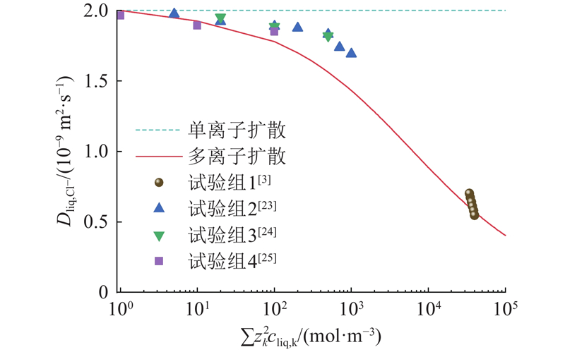
... 为了探究模型的有效性,将考虑单离子和多离子扩散时溶液内的氯离子扩散系数的计算值和试验值进行比较[3 ,23 -25 ] . 为了针对不同种类的氯盐统一比较,采用等价氯离子浓度. 以同样为1 000.0 mol/m3 的NaCl和BaCl2 溶液为例,NaCl溶液中由于Na+ 和Cl− 的浓度以及电荷数的平方均相同,根据式(8)有 $ \displaystyle\sum {z}_{k}^{2}{c}_{\mathrm{l}\mathrm{i}\mathrm{q},k}={z}_{{\mathrm{C}\mathrm{l}}^{-}}^{2}{c}_{\mathrm{l}\mathrm{i}\mathrm{q},{\mathrm{C}\mathrm{l}}^{-}}+{z}_{{\mathrm{N}\mathrm{a}}^{+}}^{2}{c}_{\mathrm{l}\mathrm{i}\mathrm{q},{\mathrm{N}\mathrm{a}}^{+}} $ 3 的NaCl溶液中Na+ 和Cl− 可以换算成浓度为2 000.0 mol/m3 的等价氯离子. 在BaCl2 溶液中,由于Cl− 和Ba2+ 浓度分别为2 000.0和1 000.0 mol/m3 ,同时Ba2+ 的电荷数平方为Cl− 的4倍. 根据式(8)有 ...
骨料对氯离子在水泥基复合材料中扩散系数的影响
3
2011
... 混凝土是由水泥浆、骨料和界面过渡区(ITZ)构成的多相复合材料. 混凝土内部的孔隙结构一方面受到水泥浆中孔隙及其空间分布的影响,另一方面与混凝土中骨料的分布有关[4 ] . 尽管骨料较致密,但骨料和水泥浆之间形成的ITZ具有较高的孔隙率. 需要考虑混凝土各相相内孔隙结构的差异对混凝土内部离子扩散系数的影响. ...
... 由于骨料较致密离子的传输难以进行,骨料中离子扩散系数通常简化为0[4 -5 ] . 水泥浆和ITZ均是多孔介质,因此可以视为由高扩散系数相介质(毛细孔内部溶液,其中离子扩散系数取水溶液中的离子扩散系数,例如室温下氯离子在无限稀释溶液中的离子扩散系数为2.03×10⁻⁹ m2 /s)和低扩散系数相介质(固相,值得注意的是水泥浆的固相中存在孔隙,例如C-S-H凝胶孔,因此离子扩散仍然可以进行)组成的两相复合材料,采用GEM理论模型对水泥浆内部离子扩散系数进行求解[28 ] . Christensen等[34 ] 研究指出,当水泥浆中的毛细孔孔隙率 $ {\varphi }_{\mathrm{c}\mathrm{e}\mathrm{m}} $ $ {t}_{\mathrm{e}\mathrm{x}\mathrm{p}} $ $ {\varphi }_{\mathrm{c}\mathrm{e}\mathrm{m}} $ $ m_{\rm{w}}/m_{\rm{c}} $ $ m $ [35 ] : ...
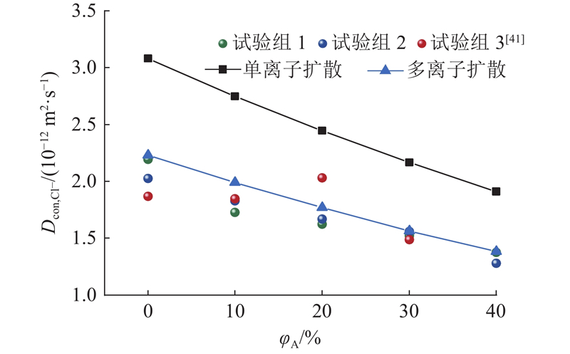
... 当仅考虑单离子扩散时,根据式(37)计算可知,毛细孔内部溶液中的氯离子的扩散系数 $ {D}_{\mathrm{l}\mathrm{i}\mathrm{q},{\mathrm{C}\mathrm{l}}^{-}} $ −9 m2 /s. 根据式(38)、(39)计算可知,水泥浆和ITZ内部的氯离子扩散系数分别为 $ {D}_{\mathrm{c}\mathrm{e}\mathrm{m},{\mathrm{C}\mathrm{l}}^{-}} $ −12 m2 /s, $ {D}_{\mathrm{I},{\mathrm{C}\mathrm{l}}^{-}} $ −12 m2 /s. $ {D}_{\mathrm{I},{\mathrm{C}\mathrm{l}}^{-}} $ $ {\mathrm{的}D}_{\mathrm{c}\mathrm{e}\mathrm{m},{\mathrm{C}\mathrm{l}}^{-}} $ 4 ,42 ,43 ]中 $D_{{\rm{I}}, {\rm{Cl}}^{-}}/D_{{\rm{cem}}, {\rm{Cl}}^{-}}$ $ {D}_{\mathrm{c}\mathrm{o}\mathrm{n},{\mathrm{C}\mathrm{l}}^{-}} $ 图6 所示. $ {D}_{\mathrm{c}\mathrm{o}\mathrm{n},{\mathrm{C}\mathrm{l}}^{-}} $ $ {\varphi }_{\mathrm{A}} $ $ {\varphi }_{\mathrm{A}} $ $ {D}_{\mathrm{c}\mathrm{o}\mathrm{n},{\mathrm{C}\mathrm{l}}^{-}} $ $ {D}_{\mathrm{c}\mathrm{o}\mathrm{n},{\mathrm{C}\mathrm{l}}^{-}} $
骨料对氯离子在水泥基复合材料中扩散系数的影响
3
2011
... 混凝土是由水泥浆、骨料和界面过渡区(ITZ)构成的多相复合材料. 混凝土内部的孔隙结构一方面受到水泥浆中孔隙及其空间分布的影响,另一方面与混凝土中骨料的分布有关[4 ] . 尽管骨料较致密,但骨料和水泥浆之间形成的ITZ具有较高的孔隙率. 需要考虑混凝土各相相内孔隙结构的差异对混凝土内部离子扩散系数的影响. ...
... 由于骨料较致密离子的传输难以进行,骨料中离子扩散系数通常简化为0[4 -5 ] . 水泥浆和ITZ均是多孔介质,因此可以视为由高扩散系数相介质(毛细孔内部溶液,其中离子扩散系数取水溶液中的离子扩散系数,例如室温下氯离子在无限稀释溶液中的离子扩散系数为2.03×10⁻⁹ m2 /s)和低扩散系数相介质(固相,值得注意的是水泥浆的固相中存在孔隙,例如C-S-H凝胶孔,因此离子扩散仍然可以进行)组成的两相复合材料,采用GEM理论模型对水泥浆内部离子扩散系数进行求解[28 ] . Christensen等[34 ] 研究指出,当水泥浆中的毛细孔孔隙率 $ {\varphi }_{\mathrm{c}\mathrm{e}\mathrm{m}} $ $ {t}_{\mathrm{e}\mathrm{x}\mathrm{p}} $ $ {\varphi }_{\mathrm{c}\mathrm{e}\mathrm{m}} $ $ m_{\rm{w}}/m_{\rm{c}} $ $ m $ [35 ] : ...
... 当仅考虑单离子扩散时,根据式(37)计算可知,毛细孔内部溶液中的氯离子的扩散系数 $ {D}_{\mathrm{l}\mathrm{i}\mathrm{q},{\mathrm{C}\mathrm{l}}^{-}} $ −9 m2 /s. 根据式(38)、(39)计算可知,水泥浆和ITZ内部的氯离子扩散系数分别为 $ {D}_{\mathrm{c}\mathrm{e}\mathrm{m},{\mathrm{C}\mathrm{l}}^{-}} $ −12 m2 /s, $ {D}_{\mathrm{I},{\mathrm{C}\mathrm{l}}^{-}} $ −12 m2 /s. $ {D}_{\mathrm{I},{\mathrm{C}\mathrm{l}}^{-}} $ $ {\mathrm{的}D}_{\mathrm{c}\mathrm{e}\mathrm{m},{\mathrm{C}\mathrm{l}}^{-}} $ 4 ,42 ,43 ]中 $D_{{\rm{I}}, {\rm{Cl}}^{-}}/D_{{\rm{cem}}, {\rm{Cl}}^{-}}$ $ {D}_{\mathrm{c}\mathrm{o}\mathrm{n},{\mathrm{C}\mathrm{l}}^{-}} $ 图6 所示. $ {D}_{\mathrm{c}\mathrm{o}\mathrm{n},{\mathrm{C}\mathrm{l}}^{-}} $ $ {\varphi }_{\mathrm{A}} $ $ {\varphi }_{\mathrm{A}} $ $ {D}_{\mathrm{c}\mathrm{o}\mathrm{n},{\mathrm{C}\mathrm{l}}^{-}} $ $ {D}_{\mathrm{c}\mathrm{o}\mathrm{n},{\mathrm{C}\mathrm{l}}^{-}} $
基于多离子传输的混凝土细微观尺度多相数值模拟
2
2018
... 基于多相复合材料理论的混凝土内部多离子的传输已成为当前混凝土内部离子传输研究的重点,在数值模拟领域中取得了进展[5 -7 ] . 关于混凝土内部离子扩散系数的理论模型研究,Thomas等[8 -12 ] 将混凝土视为均质材料,提出单相模型. 还有部分学者考虑混凝土构成组分的影响,提出由水泥浆和骨料构成的两相模型[13 -17 ] 以及由水泥浆、骨料和ITZ构成的三相模型[18 -19 ] . 这些模型中通常仅考虑单一离子扩散的情况,没有关注多种离子传输时离子种类和浓度对离子扩散系数的影响. ...
... 由于骨料较致密离子的传输难以进行,骨料中离子扩散系数通常简化为0[4 -5 ] . 水泥浆和ITZ均是多孔介质,因此可以视为由高扩散系数相介质(毛细孔内部溶液,其中离子扩散系数取水溶液中的离子扩散系数,例如室温下氯离子在无限稀释溶液中的离子扩散系数为2.03×10⁻⁹ m2 /s)和低扩散系数相介质(固相,值得注意的是水泥浆的固相中存在孔隙,例如C-S-H凝胶孔,因此离子扩散仍然可以进行)组成的两相复合材料,采用GEM理论模型对水泥浆内部离子扩散系数进行求解[28 ] . Christensen等[34 ] 研究指出,当水泥浆中的毛细孔孔隙率 $ {\varphi }_{\mathrm{c}\mathrm{e}\mathrm{m}} $ $ {t}_{\mathrm{e}\mathrm{x}\mathrm{p}} $ $ {\varphi }_{\mathrm{c}\mathrm{e}\mathrm{m}} $ $ m_{\rm{w}}/m_{\rm{c}} $ $ m $ [35 ] : ...
Finite element modeling of chloride removal from concrete by an electrochemical method
0
2000
Numerical simulation of ionic transport in cement paste under the action of externally applied electric field
1
2013
... 基于多相复合材料理论的混凝土内部多离子的传输已成为当前混凝土内部离子传输研究的重点,在数值模拟领域中取得了进展[5 -7 ] . 关于混凝土内部离子扩散系数的理论模型研究,Thomas等[8 -12 ] 将混凝土视为均质材料,提出单相模型. 还有部分学者考虑混凝土构成组分的影响,提出由水泥浆和骨料构成的两相模型[13 -17 ] 以及由水泥浆、骨料和ITZ构成的三相模型[18 -19 ] . 这些模型中通常仅考虑单一离子扩散的情况,没有关注多种离子传输时离子种类和浓度对离子扩散系数的影响. ...
Performance of slag concrete in marine environment
1
2008
... 基于多相复合材料理论的混凝土内部多离子的传输已成为当前混凝土内部离子传输研究的重点,在数值模拟领域中取得了进展[5 -7 ] . 关于混凝土内部离子扩散系数的理论模型研究,Thomas等[8 -12 ] 将混凝土视为均质材料,提出单相模型. 还有部分学者考虑混凝土构成组分的影响,提出由水泥浆和骨料构成的两相模型[13 -17 ] 以及由水泥浆、骨料和ITZ构成的三相模型[18 -19 ] . 这些模型中通常仅考虑单一离子扩散的情况,没有关注多种离子传输时离子种类和浓度对离子扩散系数的影响. ...
Characteristic service life for concrete exposed to marine environments
0
2004
Determination of chloride diffusion coefficient of concrete using open-circuit potential measurements
0
2004
Apparent diffusivity model for concrete containing supplementary cementitious materials
1
2013
... 基于多相复合材料理论的混凝土内部多离子的传输已成为当前混凝土内部离子传输研究的重点,在数值模拟领域中取得了进展[5 -7 ] . 关于混凝土内部离子扩散系数的理论模型研究,Thomas等[8 -12 ] 将混凝土视为均质材料,提出单相模型. 还有部分学者考虑混凝土构成组分的影响,提出由水泥浆和骨料构成的两相模型[13 -17 ] 以及由水泥浆、骨料和ITZ构成的三相模型[18 -19 ] . 这些模型中通常仅考虑单一离子扩散的情况,没有关注多种离子传输时离子种类和浓度对离子扩散系数的影响. ...
Effective conductivity in random porous media with convex and non-convex porosity
3
2014
... 基于多相复合材料理论的混凝土内部多离子的传输已成为当前混凝土内部离子传输研究的重点,在数值模拟领域中取得了进展[5 -7 ] . 关于混凝土内部离子扩散系数的理论模型研究,Thomas等[8 -12 ] 将混凝土视为均质材料,提出单相模型. 还有部分学者考虑混凝土构成组分的影响,提出由水泥浆和骨料构成的两相模型[13 -17 ] 以及由水泥浆、骨料和ITZ构成的三相模型[18 -19 ] . 这些模型中通常仅考虑单一离子扩散的情况,没有关注多种离子传输时离子种类和浓度对离子扩散系数的影响. ...
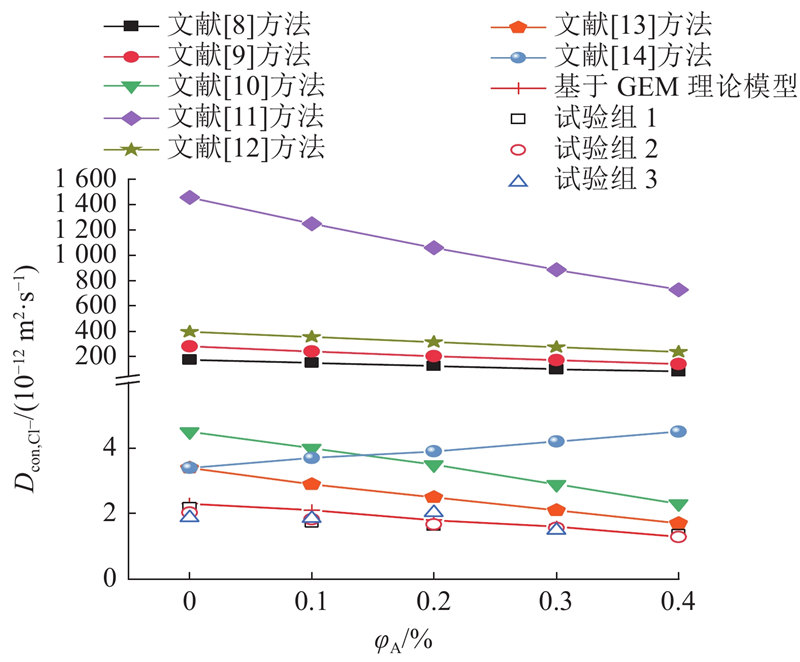
... 将本文模型和表2 中的两相[13 -17 ] 及三相[18 -19 ] 离子扩散系数模型进行对比,结果如图7 所示. 表中, $ {\varphi }_{\mathrm{l}} $ $ {\varphi }_{\mathrm{h}} $ $ {D}_{\mathrm{c}\mathrm{e}\mathrm{m}} $ $ {D}_{\mathrm{I}} $ $\varepsilon $ $ {D}_{\mathrm{c}\mathrm{e}\mathrm{m},{\mathrm{C}\mathrm{l}}^{-}} $ −12 m2 /s, $ {D}_{\mathrm{I},{\mathrm{C}\mathrm{l}}^{-}} $ −12 m2 /s. ...
... Overview of diffusion coefficient model
Tab.2 方法 公式 文献[13 ]方法 ${D}_{\mathrm{m} }={D}_{\mathrm{h} }{\left(1-{\varphi }_{\mathrm{l} }\right)}^{3/2}$ 文献[14 ]方法 $ {D}_{\mathrm{m}}={D}_{\mathrm{h}}+\dfrac{{\varphi }_{\mathrm{l}}}{\dfrac{1}{{D}_{\mathrm{l}}-{D}_{\mathrm{h}}}+\dfrac{1-{\varphi }_{\mathrm{l}}}{3{D}_{\mathrm{h}}}} $ 文献[15 ]方法 $ {D}_{\mathrm{m}}={D}_{\mathrm{h}}\mathrm{e}\mathrm{x}\mathrm{p}\left(-\dfrac{1.5{\varphi }_{\mathrm{l}}}{1-{\varphi }_{\mathrm{l}}}\right) $ 文献[16 ]方法 $ \dfrac{{D}_{\mathrm{m}}-{D}_{\mathrm{h}}}{{D}_{\mathrm{m}}+2{D}_{\mathrm{h}}}={\varphi }_{\mathrm{l}}\left(\dfrac{{D}_{\mathrm{l}}-{D}_{\mathrm{h}}}{{D}_{\mathrm{l}}+2{D}_{\mathrm{h}}}\right) $ 文献[17 ]方法 ${D}_{\mathrm{m} }=\left\{\begin{array}{c}\dfrac{ {D}_{\mathrm{h} }{D}_{\mathrm{l} } }{\left(1-{\varphi }_{\mathrm{l} }\right){D}_{\mathrm{l} }+{\varphi }_{\mathrm{l} }{D}_{\mathrm{h} } }\\ {D}_{\mathrm{h} }\left(1-{\varphi }_{\mathrm{l} }\right)+{D}_{\mathrm{l} }{\varphi }_{\mathrm{l} }\end{array}\right.$ 文献[18 ]方法 $ {D}_{\mathrm{c}\mathrm{o}\mathrm{n}}={D}_{\mathrm{c}\mathrm{e}\mathrm{m}}(0.11{\varphi }_{\mathrm{ITZ}}+1-{\varphi }_{\mathrm{A}})\dfrac{2}{2+{\varphi }_{\mathrm{A}}} $ 文献[19 ]方法 $ {D}_{\mathrm{c}\mathrm{o}\mathrm{n}}={D}_{\mathrm{c}\mathrm{e}\mathrm{m}}\left(1+\dfrac{{\varphi }_{\mathrm{A}}}{\dfrac{1-{\varphi }_{\mathrm{A}}}{3}+\dfrac{1}{{2\left({D}_{\mathrm{I}}/{D}_{\mathrm{c}\mathrm{e}\mathrm{m}}\right)}^{\varepsilon }-1}}\right) $
图 7 不同氯离子扩散系数模型的预测值对比 ...
A variational approach to the theory of the effective magnetic permeability of multiphase materials
1
1962
... Overview of diffusion coefficient model
Tab.2 方法 公式 文献[13 ]方法 ${D}_{\mathrm{m} }={D}_{\mathrm{h} }{\left(1-{\varphi }_{\mathrm{l} }\right)}^{3/2}$ 文献[14 ]方法 $ {D}_{\mathrm{m}}={D}_{\mathrm{h}}+\dfrac{{\varphi }_{\mathrm{l}}}{\dfrac{1}{{D}_{\mathrm{l}}-{D}_{\mathrm{h}}}+\dfrac{1-{\varphi }_{\mathrm{l}}}{3{D}_{\mathrm{h}}}} $ 文献[15 ]方法 $ {D}_{\mathrm{m}}={D}_{\mathrm{h}}\mathrm{e}\mathrm{x}\mathrm{p}\left(-\dfrac{1.5{\varphi }_{\mathrm{l}}}{1-{\varphi }_{\mathrm{l}}}\right) $ 文献[16 ]方法 $ \dfrac{{D}_{\mathrm{m}}-{D}_{\mathrm{h}}}{{D}_{\mathrm{m}}+2{D}_{\mathrm{h}}}={\varphi }_{\mathrm{l}}\left(\dfrac{{D}_{\mathrm{l}}-{D}_{\mathrm{h}}}{{D}_{\mathrm{l}}+2{D}_{\mathrm{h}}}\right) $ 文献[17 ]方法 ${D}_{\mathrm{m} }=\left\{\begin{array}{c}\dfrac{ {D}_{\mathrm{h} }{D}_{\mathrm{l} } }{\left(1-{\varphi }_{\mathrm{l} }\right){D}_{\mathrm{l} }+{\varphi }_{\mathrm{l} }{D}_{\mathrm{h} } }\\ {D}_{\mathrm{h} }\left(1-{\varphi }_{\mathrm{l} }\right)+{D}_{\mathrm{l} }{\varphi }_{\mathrm{l} }\end{array}\right.$ 文献[18 ]方法 $ {D}_{\mathrm{c}\mathrm{o}\mathrm{n}}={D}_{\mathrm{c}\mathrm{e}\mathrm{m}}(0.11{\varphi }_{\mathrm{ITZ}}+1-{\varphi }_{\mathrm{A}})\dfrac{2}{2+{\varphi }_{\mathrm{A}}} $ 文献[19 ]方法 $ {D}_{\mathrm{c}\mathrm{o}\mathrm{n}}={D}_{\mathrm{c}\mathrm{e}\mathrm{m}}\left(1+\dfrac{{\varphi }_{\mathrm{A}}}{\dfrac{1-{\varphi }_{\mathrm{A}}}{3}+\dfrac{1}{{2\left({D}_{\mathrm{I}}/{D}_{\mathrm{c}\mathrm{e}\mathrm{m}}\right)}^{\varepsilon }-1}}\right) $
图 7 不同氯离子扩散系数模型的预测值对比 ...
Conduction through a random suspension of spheres
1
1973
... Overview of diffusion coefficient model
Tab.2 方法 公式 文献[13 ]方法 ${D}_{\mathrm{m} }={D}_{\mathrm{h} }{\left(1-{\varphi }_{\mathrm{l} }\right)}^{3/2}$ 文献[14 ]方法 $ {D}_{\mathrm{m}}={D}_{\mathrm{h}}+\dfrac{{\varphi }_{\mathrm{l}}}{\dfrac{1}{{D}_{\mathrm{l}}-{D}_{\mathrm{h}}}+\dfrac{1-{\varphi }_{\mathrm{l}}}{3{D}_{\mathrm{h}}}} $ 文献[15 ]方法 $ {D}_{\mathrm{m}}={D}_{\mathrm{h}}\mathrm{e}\mathrm{x}\mathrm{p}\left(-\dfrac{1.5{\varphi }_{\mathrm{l}}}{1-{\varphi }_{\mathrm{l}}}\right) $ 文献[16 ]方法 $ \dfrac{{D}_{\mathrm{m}}-{D}_{\mathrm{h}}}{{D}_{\mathrm{m}}+2{D}_{\mathrm{h}}}={\varphi }_{\mathrm{l}}\left(\dfrac{{D}_{\mathrm{l}}-{D}_{\mathrm{h}}}{{D}_{\mathrm{l}}+2{D}_{\mathrm{h}}}\right) $ 文献[17 ]方法 ${D}_{\mathrm{m} }=\left\{\begin{array}{c}\dfrac{ {D}_{\mathrm{h} }{D}_{\mathrm{l} } }{\left(1-{\varphi }_{\mathrm{l} }\right){D}_{\mathrm{l} }+{\varphi }_{\mathrm{l} }{D}_{\mathrm{h} } }\\ {D}_{\mathrm{h} }\left(1-{\varphi }_{\mathrm{l} }\right)+{D}_{\mathrm{l} }{\varphi }_{\mathrm{l} }\end{array}\right.$ 文献[18 ]方法 $ {D}_{\mathrm{c}\mathrm{o}\mathrm{n}}={D}_{\mathrm{c}\mathrm{e}\mathrm{m}}(0.11{\varphi }_{\mathrm{ITZ}}+1-{\varphi }_{\mathrm{A}})\dfrac{2}{2+{\varphi }_{\mathrm{A}}} $ 文献[19 ]方法 $ {D}_{\mathrm{c}\mathrm{o}\mathrm{n}}={D}_{\mathrm{c}\mathrm{e}\mathrm{m}}\left(1+\dfrac{{\varphi }_{\mathrm{A}}}{\dfrac{1-{\varphi }_{\mathrm{A}}}{3}+\dfrac{1}{{2\left({D}_{\mathrm{I}}/{D}_{\mathrm{c}\mathrm{e}\mathrm{m}}\right)}^{\varepsilon }-1}}\right) $
图 7 不同氯离子扩散系数模型的预测值对比 ...
Maxwell-Garnett mixing rule in the presence of multiple scattering: derivation and accuracy
1
2005
... Overview of diffusion coefficient model
Tab.2 方法 公式 文献[13 ]方法 ${D}_{\mathrm{m} }={D}_{\mathrm{h} }{\left(1-{\varphi }_{\mathrm{l} }\right)}^{3/2}$ 文献[14 ]方法 $ {D}_{\mathrm{m}}={D}_{\mathrm{h}}+\dfrac{{\varphi }_{\mathrm{l}}}{\dfrac{1}{{D}_{\mathrm{l}}-{D}_{\mathrm{h}}}+\dfrac{1-{\varphi }_{\mathrm{l}}}{3{D}_{\mathrm{h}}}} $ 文献[15 ]方法 $ {D}_{\mathrm{m}}={D}_{\mathrm{h}}\mathrm{e}\mathrm{x}\mathrm{p}\left(-\dfrac{1.5{\varphi }_{\mathrm{l}}}{1-{\varphi }_{\mathrm{l}}}\right) $ 文献[16 ]方法 $ \dfrac{{D}_{\mathrm{m}}-{D}_{\mathrm{h}}}{{D}_{\mathrm{m}}+2{D}_{\mathrm{h}}}={\varphi }_{\mathrm{l}}\left(\dfrac{{D}_{\mathrm{l}}-{D}_{\mathrm{h}}}{{D}_{\mathrm{l}}+2{D}_{\mathrm{h}}}\right) $ 文献[17 ]方法 ${D}_{\mathrm{m} }=\left\{\begin{array}{c}\dfrac{ {D}_{\mathrm{h} }{D}_{\mathrm{l} } }{\left(1-{\varphi }_{\mathrm{l} }\right){D}_{\mathrm{l} }+{\varphi }_{\mathrm{l} }{D}_{\mathrm{h} } }\\ {D}_{\mathrm{h} }\left(1-{\varphi }_{\mathrm{l} }\right)+{D}_{\mathrm{l} }{\varphi }_{\mathrm{l} }\end{array}\right.$ 文献[18 ]方法 $ {D}_{\mathrm{c}\mathrm{o}\mathrm{n}}={D}_{\mathrm{c}\mathrm{e}\mathrm{m}}(0.11{\varphi }_{\mathrm{ITZ}}+1-{\varphi }_{\mathrm{A}})\dfrac{2}{2+{\varphi }_{\mathrm{A}}} $ 文献[19 ]方法 $ {D}_{\mathrm{c}\mathrm{o}\mathrm{n}}={D}_{\mathrm{c}\mathrm{e}\mathrm{m}}\left(1+\dfrac{{\varphi }_{\mathrm{A}}}{\dfrac{1-{\varphi }_{\mathrm{A}}}{3}+\dfrac{1}{{2\left({D}_{\mathrm{I}}/{D}_{\mathrm{c}\mathrm{e}\mathrm{m}}\right)}^{\varepsilon }-1}}\right) $
图 7 不同氯离子扩散系数模型的预测值对比 ...
Modeling the influence of particulate geometry on the thermal conductivity of composites
3
2014
... 基于多相复合材料理论的混凝土内部多离子的传输已成为当前混凝土内部离子传输研究的重点,在数值模拟领域中取得了进展[5 -7 ] . 关于混凝土内部离子扩散系数的理论模型研究,Thomas等[8 -12 ] 将混凝土视为均质材料,提出单相模型. 还有部分学者考虑混凝土构成组分的影响,提出由水泥浆和骨料构成的两相模型[13 -17 ] 以及由水泥浆、骨料和ITZ构成的三相模型[18 -19 ] . 这些模型中通常仅考虑单一离子扩散的情况,没有关注多种离子传输时离子种类和浓度对离子扩散系数的影响. ...
... 将本文模型和表2 中的两相[13 -17 ] 及三相[18 -19 ] 离子扩散系数模型进行对比,结果如图7 所示. 表中, $ {\varphi }_{\mathrm{l}} $ $ {\varphi }_{\mathrm{h}} $ $ {D}_{\mathrm{c}\mathrm{e}\mathrm{m}} $ $ {D}_{\mathrm{I}} $ $\varepsilon $ $ {D}_{\mathrm{c}\mathrm{e}\mathrm{m},{\mathrm{C}\mathrm{l}}^{-}} $ −12 m2 /s, $ {D}_{\mathrm{I},{\mathrm{C}\mathrm{l}}^{-}} $ −12 m2 /s. ...
... Overview of diffusion coefficient model
Tab.2 方法 公式 文献[13 ]方法 ${D}_{\mathrm{m} }={D}_{\mathrm{h} }{\left(1-{\varphi }_{\mathrm{l} }\right)}^{3/2}$ 文献[14 ]方法 $ {D}_{\mathrm{m}}={D}_{\mathrm{h}}+\dfrac{{\varphi }_{\mathrm{l}}}{\dfrac{1}{{D}_{\mathrm{l}}-{D}_{\mathrm{h}}}+\dfrac{1-{\varphi }_{\mathrm{l}}}{3{D}_{\mathrm{h}}}} $ 文献[15 ]方法 $ {D}_{\mathrm{m}}={D}_{\mathrm{h}}\mathrm{e}\mathrm{x}\mathrm{p}\left(-\dfrac{1.5{\varphi }_{\mathrm{l}}}{1-{\varphi }_{\mathrm{l}}}\right) $ 文献[16 ]方法 $ \dfrac{{D}_{\mathrm{m}}-{D}_{\mathrm{h}}}{{D}_{\mathrm{m}}+2{D}_{\mathrm{h}}}={\varphi }_{\mathrm{l}}\left(\dfrac{{D}_{\mathrm{l}}-{D}_{\mathrm{h}}}{{D}_{\mathrm{l}}+2{D}_{\mathrm{h}}}\right) $ 文献[17 ]方法 ${D}_{\mathrm{m} }=\left\{\begin{array}{c}\dfrac{ {D}_{\mathrm{h} }{D}_{\mathrm{l} } }{\left(1-{\varphi }_{\mathrm{l} }\right){D}_{\mathrm{l} }+{\varphi }_{\mathrm{l} }{D}_{\mathrm{h} } }\\ {D}_{\mathrm{h} }\left(1-{\varphi }_{\mathrm{l} }\right)+{D}_{\mathrm{l} }{\varphi }_{\mathrm{l} }\end{array}\right.$ 文献[18 ]方法 $ {D}_{\mathrm{c}\mathrm{o}\mathrm{n}}={D}_{\mathrm{c}\mathrm{e}\mathrm{m}}(0.11{\varphi }_{\mathrm{ITZ}}+1-{\varphi }_{\mathrm{A}})\dfrac{2}{2+{\varphi }_{\mathrm{A}}} $ 文献[19 ]方法 $ {D}_{\mathrm{c}\mathrm{o}\mathrm{n}}={D}_{\mathrm{c}\mathrm{e}\mathrm{m}}\left(1+\dfrac{{\varphi }_{\mathrm{A}}}{\dfrac{1-{\varphi }_{\mathrm{A}}}{3}+\dfrac{1}{{2\left({D}_{\mathrm{I}}/{D}_{\mathrm{c}\mathrm{e}\mathrm{m}}\right)}^{\varepsilon }-1}}\right) $
图 7 不同氯离子扩散系数模型的预测值对比 ...
Influence of aggregates on chloride diffusion coefficient into mortar
3
2003
... 基于多相复合材料理论的混凝土内部多离子的传输已成为当前混凝土内部离子传输研究的重点,在数值模拟领域中取得了进展[5 -7 ] . 关于混凝土内部离子扩散系数的理论模型研究,Thomas等[8 -12 ] 将混凝土视为均质材料,提出单相模型. 还有部分学者考虑混凝土构成组分的影响,提出由水泥浆和骨料构成的两相模型[13 -17 ] 以及由水泥浆、骨料和ITZ构成的三相模型[18 -19 ] . 这些模型中通常仅考虑单一离子扩散的情况,没有关注多种离子传输时离子种类和浓度对离子扩散系数的影响. ...
... 将本文模型和表2 中的两相[13 -17 ] 及三相[18 -19 ] 离子扩散系数模型进行对比,结果如图7 所示. 表中, $ {\varphi }_{\mathrm{l}} $ $ {\varphi }_{\mathrm{h}} $ $ {D}_{\mathrm{c}\mathrm{e}\mathrm{m}} $ $ {D}_{\mathrm{I}} $ $\varepsilon $ $ {D}_{\mathrm{c}\mathrm{e}\mathrm{m},{\mathrm{C}\mathrm{l}}^{-}} $ −12 m2 /s, $ {D}_{\mathrm{I},{\mathrm{C}\mathrm{l}}^{-}} $ −12 m2 /s. ...
... Overview of diffusion coefficient model
Tab.2 方法 公式 文献[13 ]方法 ${D}_{\mathrm{m} }={D}_{\mathrm{h} }{\left(1-{\varphi }_{\mathrm{l} }\right)}^{3/2}$ 文献[14 ]方法 $ {D}_{\mathrm{m}}={D}_{\mathrm{h}}+\dfrac{{\varphi }_{\mathrm{l}}}{\dfrac{1}{{D}_{\mathrm{l}}-{D}_{\mathrm{h}}}+\dfrac{1-{\varphi }_{\mathrm{l}}}{3{D}_{\mathrm{h}}}} $ 文献[15 ]方法 $ {D}_{\mathrm{m}}={D}_{\mathrm{h}}\mathrm{e}\mathrm{x}\mathrm{p}\left(-\dfrac{1.5{\varphi }_{\mathrm{l}}}{1-{\varphi }_{\mathrm{l}}}\right) $ 文献[16 ]方法 $ \dfrac{{D}_{\mathrm{m}}-{D}_{\mathrm{h}}}{{D}_{\mathrm{m}}+2{D}_{\mathrm{h}}}={\varphi }_{\mathrm{l}}\left(\dfrac{{D}_{\mathrm{l}}-{D}_{\mathrm{h}}}{{D}_{\mathrm{l}}+2{D}_{\mathrm{h}}}\right) $ 文献[17 ]方法 ${D}_{\mathrm{m} }=\left\{\begin{array}{c}\dfrac{ {D}_{\mathrm{h} }{D}_{\mathrm{l} } }{\left(1-{\varphi }_{\mathrm{l} }\right){D}_{\mathrm{l} }+{\varphi }_{\mathrm{l} }{D}_{\mathrm{h} } }\\ {D}_{\mathrm{h} }\left(1-{\varphi }_{\mathrm{l} }\right)+{D}_{\mathrm{l} }{\varphi }_{\mathrm{l} }\end{array}\right.$ 文献[18 ]方法 $ {D}_{\mathrm{c}\mathrm{o}\mathrm{n}}={D}_{\mathrm{c}\mathrm{e}\mathrm{m}}(0.11{\varphi }_{\mathrm{ITZ}}+1-{\varphi }_{\mathrm{A}})\dfrac{2}{2+{\varphi }_{\mathrm{A}}} $ 文献[19 ]方法 $ {D}_{\mathrm{c}\mathrm{o}\mathrm{n}}={D}_{\mathrm{c}\mathrm{e}\mathrm{m}}\left(1+\dfrac{{\varphi }_{\mathrm{A}}}{\dfrac{1-{\varphi }_{\mathrm{A}}}{3}+\dfrac{1}{{2\left({D}_{\mathrm{I}}/{D}_{\mathrm{c}\mathrm{e}\mathrm{m}}\right)}^{\varepsilon }-1}}\right) $
图 7 不同氯离子扩散系数模型的预测值对比 ...
Thin interphase/imperfect interface in conduction
3
2001
... 基于多相复合材料理论的混凝土内部多离子的传输已成为当前混凝土内部离子传输研究的重点,在数值模拟领域中取得了进展[5 -7 ] . 关于混凝土内部离子扩散系数的理论模型研究,Thomas等[8 -12 ] 将混凝土视为均质材料,提出单相模型. 还有部分学者考虑混凝土构成组分的影响,提出由水泥浆和骨料构成的两相模型[13 -17 ] 以及由水泥浆、骨料和ITZ构成的三相模型[18 -19 ] . 这些模型中通常仅考虑单一离子扩散的情况,没有关注多种离子传输时离子种类和浓度对离子扩散系数的影响. ...
... 将本文模型和表2 中的两相[13 -17 ] 及三相[18 -19 ] 离子扩散系数模型进行对比,结果如图7 所示. 表中, $ {\varphi }_{\mathrm{l}} $ $ {\varphi }_{\mathrm{h}} $ $ {D}_{\mathrm{c}\mathrm{e}\mathrm{m}} $ $ {D}_{\mathrm{I}} $ $\varepsilon $ $ {D}_{\mathrm{c}\mathrm{e}\mathrm{m},{\mathrm{C}\mathrm{l}}^{-}} $ −12 m2 /s, $ {D}_{\mathrm{I},{\mathrm{C}\mathrm{l}}^{-}} $ −12 m2 /s. ...
... Overview of diffusion coefficient model
Tab.2 方法 公式 文献[13 ]方法 ${D}_{\mathrm{m} }={D}_{\mathrm{h} }{\left(1-{\varphi }_{\mathrm{l} }\right)}^{3/2}$ 文献[14 ]方法 $ {D}_{\mathrm{m}}={D}_{\mathrm{h}}+\dfrac{{\varphi }_{\mathrm{l}}}{\dfrac{1}{{D}_{\mathrm{l}}-{D}_{\mathrm{h}}}+\dfrac{1-{\varphi }_{\mathrm{l}}}{3{D}_{\mathrm{h}}}} $ 文献[15 ]方法 $ {D}_{\mathrm{m}}={D}_{\mathrm{h}}\mathrm{e}\mathrm{x}\mathrm{p}\left(-\dfrac{1.5{\varphi }_{\mathrm{l}}}{1-{\varphi }_{\mathrm{l}}}\right) $ 文献[16 ]方法 $ \dfrac{{D}_{\mathrm{m}}-{D}_{\mathrm{h}}}{{D}_{\mathrm{m}}+2{D}_{\mathrm{h}}}={\varphi }_{\mathrm{l}}\left(\dfrac{{D}_{\mathrm{l}}-{D}_{\mathrm{h}}}{{D}_{\mathrm{l}}+2{D}_{\mathrm{h}}}\right) $ 文献[17 ]方法 ${D}_{\mathrm{m} }=\left\{\begin{array}{c}\dfrac{ {D}_{\mathrm{h} }{D}_{\mathrm{l} } }{\left(1-{\varphi }_{\mathrm{l} }\right){D}_{\mathrm{l} }+{\varphi }_{\mathrm{l} }{D}_{\mathrm{h} } }\\ {D}_{\mathrm{h} }\left(1-{\varphi }_{\mathrm{l} }\right)+{D}_{\mathrm{l} }{\varphi }_{\mathrm{l} }\end{array}\right.$ 文献[18 ]方法 $ {D}_{\mathrm{c}\mathrm{o}\mathrm{n}}={D}_{\mathrm{c}\mathrm{e}\mathrm{m}}(0.11{\varphi }_{\mathrm{ITZ}}+1-{\varphi }_{\mathrm{A}})\dfrac{2}{2+{\varphi }_{\mathrm{A}}} $ 文献[19 ]方法 $ {D}_{\mathrm{c}\mathrm{o}\mathrm{n}}={D}_{\mathrm{c}\mathrm{e}\mathrm{m}}\left(1+\dfrac{{\varphi }_{\mathrm{A}}}{\dfrac{1-{\varphi }_{\mathrm{A}}}{3}+\dfrac{1}{{2\left({D}_{\mathrm{I}}/{D}_{\mathrm{c}\mathrm{e}\mathrm{m}}\right)}^{\varepsilon }-1}}\right) $
图 7 不同氯离子扩散系数模型的预测值对比 ...
Application of the Nernst-Einstein equation to concrete
2
1997
... 离子在混凝土内部传输的本质是带电粒子在多孔介质的孔隙内部的溶液中传质的过程. 根据Nernst-Einstein方程可知,多离子传输时溶液中离子的扩散系数[20 ] 为 ...
... 电导率的分项系数 $ {L}_{k} $ [20 ] 计算: ...
Estimating the electrical conductivity of cement paste pore solutions from OH? , K+ and Na+ concentrations
2
2003
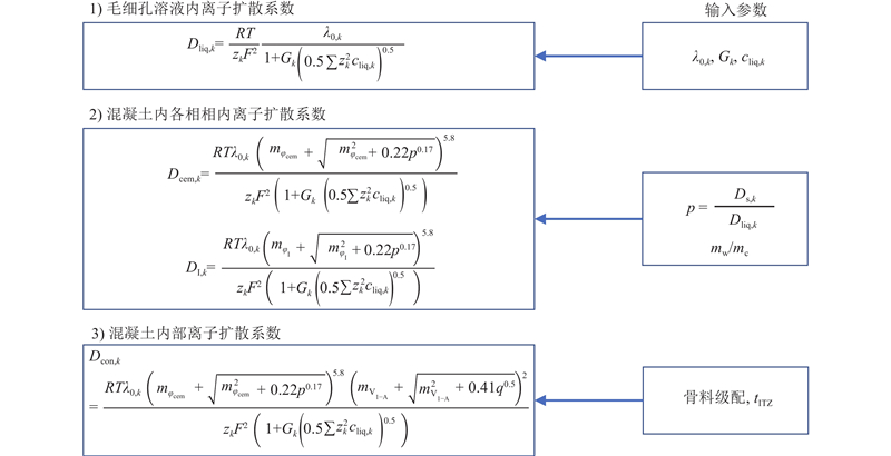
... 为了研究多离子传输对溶液内离子扩散系数的影响,分以下2种情况对离子扩散系数进行讨论:1)考虑单离子的扩散;2)考虑多离子的扩散. 以含氯离子的溶液为例,Cl− 的电导率参数为 $ {{z}_{k}\lambda }_{0,k} $ −3 S·m2 /mol, $ {G}_{k} $ −0.5[22 ] . ...
... 模型中参数取值如下: $ {\lambda }_{0,{\mathrm{C}\mathrm{l}}^{-}} $ −3 S·m2 /mol和 $ {G}_{{\mathrm{C}\mathrm{l}}^{-}} $ −0.5[22 ] , $ {c}_{\mathrm{l}\mathrm{i}\mathrm{q},{\mathrm{C}\mathrm{l}}^{-}}={c}_{\mathrm{l}\mathrm{i}\mathrm{q},{\mathrm{N}\mathrm{a}}^{+}} $ 3 , $ p = $ 1 ×10⁻⁵[28 ] , $ m_{\rm{w}}/m_{\rm{c}} $ $ {t}_{\mathrm{I}\mathrm{T}\mathrm{Z}} $
The self-diffusion coefficients of the ions in aqueous sodium chloride and sodium sulfate at 25 ℃
1
1952
... 为了探究模型的有效性,将考虑单离子和多离子扩散时溶液内的氯离子扩散系数的计算值和试验值进行比较[3 ,23 -25 ] . 为了针对不同种类的氯盐统一比较,采用等价氯离子浓度. 以同样为1 000.0 mol/m3 的NaCl和BaCl2 溶液为例,NaCl溶液中由于Na+ 和Cl− 的浓度以及电荷数的平方均相同,根据式(8)有 $ \displaystyle\sum {z}_{k}^{2}{c}_{\mathrm{l}\mathrm{i}\mathrm{q},k}={z}_{{\mathrm{C}\mathrm{l}}^{-}}^{2}{c}_{\mathrm{l}\mathrm{i}\mathrm{q},{\mathrm{C}\mathrm{l}}^{-}}+{z}_{{\mathrm{N}\mathrm{a}}^{+}}^{2}{c}_{\mathrm{l}\mathrm{i}\mathrm{q},{\mathrm{N}\mathrm{a}}^{+}} $ 3 的NaCl溶液中Na+ 和Cl− 可以换算成浓度为2 000.0 mol/m3 的等价氯离子. 在BaCl2 溶液中,由于Cl− 和Ba2+ 浓度分别为2 000.0和1 000.0 mol/m3 ,同时Ba2+ 的电荷数平方为Cl− 的4倍. 根据式(8)有 ...
The diffusion of potassium chloride in aqueous solution
0
1935
Diffusion coefficients in aqueous solutions of potassium chloride at high and low concentrations
1
1998
... 为了探究模型的有效性,将考虑单离子和多离子扩散时溶液内的氯离子扩散系数的计算值和试验值进行比较[3 ,23 -25 ] . 为了针对不同种类的氯盐统一比较,采用等价氯离子浓度. 以同样为1 000.0 mol/m3 的NaCl和BaCl2 溶液为例,NaCl溶液中由于Na+ 和Cl− 的浓度以及电荷数的平方均相同,根据式(8)有 $ \displaystyle\sum {z}_{k}^{2}{c}_{\mathrm{l}\mathrm{i}\mathrm{q},k}={z}_{{\mathrm{C}\mathrm{l}}^{-}}^{2}{c}_{\mathrm{l}\mathrm{i}\mathrm{q},{\mathrm{C}\mathrm{l}}^{-}}+{z}_{{\mathrm{N}\mathrm{a}}^{+}}^{2}{c}_{\mathrm{l}\mathrm{i}\mathrm{q},{\mathrm{N}\mathrm{a}}^{+}} $ 3 的NaCl溶液中Na+ 和Cl− 可以换算成浓度为2 000.0 mol/m3 的等价氯离子. 在BaCl2 溶液中,由于Cl− 和Ba2+ 浓度分别为2 000.0和1 000.0 mol/m3 ,同时Ba2+ 的电荷数平方为Cl− 的4倍. 根据式(8)有 ...
1
... 如图1 所示,仅考虑单离子扩散,氯离子扩散系数恒为2.00×10⁻⁹ m2 /s,和稀溶液中的氯离子扩散系数2.03×10−9 m2 /s高度符合[26 ] . 考虑多离子扩散,当等价氯离子浓度较低时,氯离子扩散系数接近2.00×10⁻⁹ m2 /s. 氯离子扩散系数随着等价氯离子浓度的上升而持续下降,当等价氯离子浓度从1.0 mol/m3 上升至1 000.0 mol/m3 时,氯离子扩散系数下降了大约25%. 试验数据表明,氯离子扩散系数随着等价氯离子浓度的上升而持续下降. 当等价氯离子浓度从1.0 mol/m3 上升至1 000.0 mol/m3 时,氯离子扩散系数下降了16%;因此,溶液中离子浓度对扩散系数有着明显的影响,两者为负相关关系. ...
Electrical resistivity of composites
3
1990
... 关于两相复合材料的性质计算,Mclachlan等[27 ] 提出GEM理论模型: ...
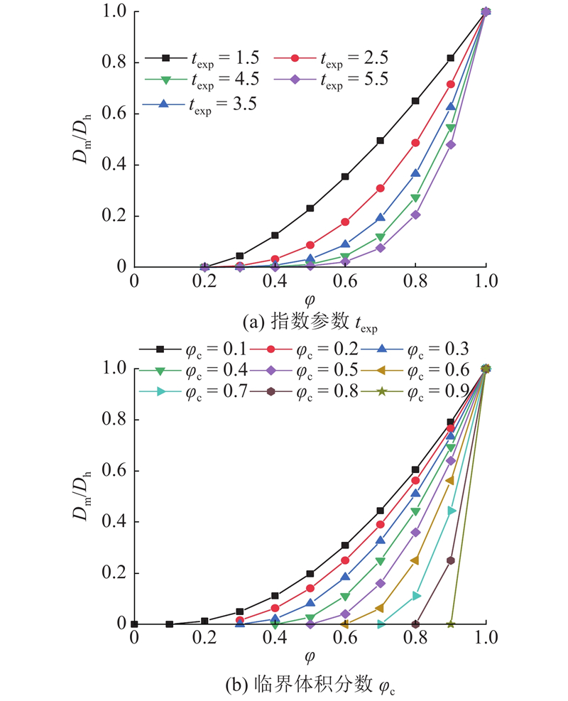
... 在GEM理论模型中,指数参数 $ {t}_{\mathrm{e}\mathrm{x}\mathrm{p}} $ $ {\varphi }_{\mathrm{c}} $ $ {t}_{\mathrm{e}\mathrm{x}\mathrm{p}} $ $ {\varphi }_{\mathrm{c}} $ $ {D}_{\mathrm{m}} $ $ {t}_{\mathrm{e}\mathrm{x}\mathrm{p}} $ [27 , 29 ] 采用连续渗流理论研究发现,绝大部分复合材料中 $ {t}_{\mathrm{e}\mathrm{x}\mathrm{p}} $ $ {t}_{\mathrm{e}\mathrm{x}\mathrm{p}} $ [30 ] 研究薄片状的介质,指出针对这种介质 $ {\mathrm{的}t}_{\mathrm{e}\mathrm{x}\mathrm{p}} $ $ {\varphi }_{\mathrm{c}} $ [31 ] 针对球状介质进行研究,指出 $ {\varphi }_{\mathrm{c}} $ $ {\varphi }_{\mathrm{c}}\mathrm{的} $ [32 ] 利用模拟的方法,指出 $ {\varphi }_{\mathrm{c}} $ [33 ] 利用连续渗流理论研究发现,在介质的形状分别为四面体、六面体和球体等情况下, $ {\varphi }_{\mathrm{c}} $
... 水泥浆和骨料之间形成ITZ,可以看作骨料被ITZ相包裹,将骨料和ITZ视为骨料-ITZ相. 骨料形状简化为球体,可以采用Bruggeman非对称介质理论(该理论是GEM理论的特殊形式[27 ] )计算骨料-ITZ相内的离子扩散系数 $ {D}_{\mathrm{I}-\mathrm{A},k}$
Prediction of diffusivity of concrete based on simple analytic equations
5
2004
... 式(10)的解析解[28 ] 为 ...
... 根据式(1),有[28 ] ...
... 式(10)可以改写为[28 ] ...
... 由于骨料较致密离子的传输难以进行,骨料中离子扩散系数通常简化为0[4 -5 ] . 水泥浆和ITZ均是多孔介质,因此可以视为由高扩散系数相介质(毛细孔内部溶液,其中离子扩散系数取水溶液中的离子扩散系数,例如室温下氯离子在无限稀释溶液中的离子扩散系数为2.03×10⁻⁹ m2 /s)和低扩散系数相介质(固相,值得注意的是水泥浆的固相中存在孔隙,例如C-S-H凝胶孔,因此离子扩散仍然可以进行)组成的两相复合材料,采用GEM理论模型对水泥浆内部离子扩散系数进行求解[28 ] . Christensen等[34 ] 研究指出,当水泥浆中的毛细孔孔隙率 $ {\varphi }_{\mathrm{c}\mathrm{e}\mathrm{m}} $ $ {t}_{\mathrm{e}\mathrm{x}\mathrm{p}} $ $ {\varphi }_{\mathrm{c}\mathrm{e}\mathrm{m}} $ $ m_{\rm{w}}/m_{\rm{c}} $ $ m $ [35 ] : ...
... 模型中参数取值如下: $ {\lambda }_{0,{\mathrm{C}\mathrm{l}}^{-}} $ −3 S·m2 /mol和 $ {G}_{{\mathrm{C}\mathrm{l}}^{-}} $ −0.5[22 ] , $ {c}_{\mathrm{l}\mathrm{i}\mathrm{q},{\mathrm{C}\mathrm{l}}^{-}}={c}_{\mathrm{l}\mathrm{i}\mathrm{q},{\mathrm{N}\mathrm{a}}^{+}} $ 3 , $ p = $ 1 ×10⁻⁵[28 ] , $ m_{\rm{w}}/m_{\rm{c}} $ $ {t}_{\mathrm{I}\mathrm{T}\mathrm{Z}} $
Percolation, statistical topography, and transport in random media
1
1992
... 在GEM理论模型中,指数参数 $ {t}_{\mathrm{e}\mathrm{x}\mathrm{p}} $ $ {\varphi }_{\mathrm{c}} $ $ {t}_{\mathrm{e}\mathrm{x}\mathrm{p}} $ $ {\varphi }_{\mathrm{c}} $ $ {D}_{\mathrm{m}} $ $ {t}_{\mathrm{e}\mathrm{x}\mathrm{p}} $ [27 , 29 ] 采用连续渗流理论研究发现,绝大部分复合材料中 $ {t}_{\mathrm{e}\mathrm{x}\mathrm{p}} $ $ {t}_{\mathrm{e}\mathrm{x}\mathrm{p}} $ [30 ] 研究薄片状的介质,指出针对这种介质 $ {\mathrm{的}t}_{\mathrm{e}\mathrm{x}\mathrm{p}} $ $ {\varphi }_{\mathrm{c}} $ [31 ] 针对球状介质进行研究,指出 $ {\varphi }_{\mathrm{c}} $ $ {\varphi }_{\mathrm{c}}\mathrm{的} $ [32 ] 利用模拟的方法,指出 $ {\varphi }_{\mathrm{c}} $ [33 ] 利用连续渗流理论研究发现,在介质的形状分别为四面体、六面体和球体等情况下, $ {\varphi }_{\mathrm{c}} $
Electrical conductivity and fiber orientation of poly (methyl methacrylate)/carbon fiber composite sheets with various thickness
1
2020
... 在GEM理论模型中,指数参数 $ {t}_{\mathrm{e}\mathrm{x}\mathrm{p}} $ $ {\varphi }_{\mathrm{c}} $ $ {t}_{\mathrm{e}\mathrm{x}\mathrm{p}} $ $ {\varphi }_{\mathrm{c}} $ $ {D}_{\mathrm{m}} $ $ {t}_{\mathrm{e}\mathrm{x}\mathrm{p}} $ [27 , 29 ] 采用连续渗流理论研究发现,绝大部分复合材料中 $ {t}_{\mathrm{e}\mathrm{x}\mathrm{p}} $ $ {t}_{\mathrm{e}\mathrm{x}\mathrm{p}} $ [30 ] 研究薄片状的介质,指出针对这种介质 $ {\mathrm{的}t}_{\mathrm{e}\mathrm{x}\mathrm{p}} $ $ {\varphi }_{\mathrm{c}} $ [31 ] 针对球状介质进行研究,指出 $ {\varphi }_{\mathrm{c}} $ $ {\varphi }_{\mathrm{c}}\mathrm{的} $ [32 ] 利用模拟的方法,指出 $ {\varphi }_{\mathrm{c}} $ [33 ] 利用连续渗流理论研究发现,在介质的形状分别为四面体、六面体和球体等情况下, $ {\varphi }_{\mathrm{c}} $
Effect of particle morphologies on the percolation of particulate porous media: a study of superballs
1
2018
... 在GEM理论模型中,指数参数 $ {t}_{\mathrm{e}\mathrm{x}\mathrm{p}} $ $ {\varphi }_{\mathrm{c}} $ $ {t}_{\mathrm{e}\mathrm{x}\mathrm{p}} $ $ {\varphi }_{\mathrm{c}} $ $ {D}_{\mathrm{m}} $ $ {t}_{\mathrm{e}\mathrm{x}\mathrm{p}} $ [27 , 29 ] 采用连续渗流理论研究发现,绝大部分复合材料中 $ {t}_{\mathrm{e}\mathrm{x}\mathrm{p}} $ $ {t}_{\mathrm{e}\mathrm{x}\mathrm{p}} $ [30 ] 研究薄片状的介质,指出针对这种介质 $ {\mathrm{的}t}_{\mathrm{e}\mathrm{x}\mathrm{p}} $ $ {\varphi }_{\mathrm{c}} $ [31 ] 针对球状介质进行研究,指出 $ {\varphi }_{\mathrm{c}} $ $ {\varphi }_{\mathrm{c}}\mathrm{的} $ [32 ] 利用模拟的方法,指出 $ {\varphi }_{\mathrm{c}} $ [33 ] 利用连续渗流理论研究发现,在介质的形状分别为四面体、六面体和球体等情况下, $ {\varphi }_{\mathrm{c}} $
Effects of the pore shape polydispersity on the percolation threshold and diffusivity of porous composites: theoretical and numerical studies
1
2021
... 在GEM理论模型中,指数参数 $ {t}_{\mathrm{e}\mathrm{x}\mathrm{p}} $ $ {\varphi }_{\mathrm{c}} $ $ {t}_{\mathrm{e}\mathrm{x}\mathrm{p}} $ $ {\varphi }_{\mathrm{c}} $ $ {D}_{\mathrm{m}} $ $ {t}_{\mathrm{e}\mathrm{x}\mathrm{p}} $ [27 , 29 ] 采用连续渗流理论研究发现,绝大部分复合材料中 $ {t}_{\mathrm{e}\mathrm{x}\mathrm{p}} $ $ {t}_{\mathrm{e}\mathrm{x}\mathrm{p}} $ [30 ] 研究薄片状的介质,指出针对这种介质 $ {\mathrm{的}t}_{\mathrm{e}\mathrm{x}\mathrm{p}} $ $ {\varphi }_{\mathrm{c}} $ [31 ] 针对球状介质进行研究,指出 $ {\varphi }_{\mathrm{c}} $ $ {\varphi }_{\mathrm{c}}\mathrm{的} $ [32 ] 利用模拟的方法,指出 $ {\varphi }_{\mathrm{c}} $ [33 ] 利用连续渗流理论研究发现,在介质的形状分别为四面体、六面体和球体等情况下, $ {\varphi }_{\mathrm{c}} $
n-Phase micromechanical framework for the conductivity and elastic modulus of particulate composites: design to microencapsulated phase change materials (MPCMs)-cementitious composites
2
2018
... 在GEM理论模型中,指数参数 $ {t}_{\mathrm{e}\mathrm{x}\mathrm{p}} $ $ {\varphi }_{\mathrm{c}} $ $ {t}_{\mathrm{e}\mathrm{x}\mathrm{p}} $ $ {\varphi }_{\mathrm{c}} $ $ {D}_{\mathrm{m}} $ $ {t}_{\mathrm{e}\mathrm{x}\mathrm{p}} $ [27 , 29 ] 采用连续渗流理论研究发现,绝大部分复合材料中 $ {t}_{\mathrm{e}\mathrm{x}\mathrm{p}} $ $ {t}_{\mathrm{e}\mathrm{x}\mathrm{p}} $ [30 ] 研究薄片状的介质,指出针对这种介质 $ {\mathrm{的}t}_{\mathrm{e}\mathrm{x}\mathrm{p}} $ $ {\varphi }_{\mathrm{c}} $ [31 ] 针对球状介质进行研究,指出 $ {\varphi }_{\mathrm{c}} $ $ {\varphi }_{\mathrm{c}}\mathrm{的} $ [32 ] 利用模拟的方法,指出 $ {\varphi }_{\mathrm{c}} $ [33 ] 利用连续渗流理论研究发现,在介质的形状分别为四面体、六面体和球体等情况下, $ {\varphi }_{\mathrm{c}} $
... 骨料-ITZ相散布在水泥浆中,将混凝土简化为两相复合材料,可以采用GEM理论计算混凝土内部离子扩散系数. 目前,对于混凝土的GEM理论参数研究较少,但是根据Xu等[33 ] 的数值模拟研究可知,在三维空间中,当介质形状为球体时, $ {t}_{\mathrm{e}\mathrm{x}\mathrm{p}}=2 $ $ {\varphi }_{\mathrm{c}}=0.29 $ . 令骨料-ITZ相和水泥浆中离子扩散系数的比值 $q ={{D}_{\mathrm{I}-\mathrm{A},k}}/{{D}_{\mathrm{c}\mathrm{e}\mathrm{m},k}}$ $ {D}_{\mathrm{c}\mathrm{o}\mathrm{n},k} $
Impedance spectroscopy of hydrating cement-based materials: measurement, interpretation, and application
1
1994
... 由于骨料较致密离子的传输难以进行,骨料中离子扩散系数通常简化为0[4 -5 ] . 水泥浆和ITZ均是多孔介质,因此可以视为由高扩散系数相介质(毛细孔内部溶液,其中离子扩散系数取水溶液中的离子扩散系数,例如室温下氯离子在无限稀释溶液中的离子扩散系数为2.03×10⁻⁹ m2 /s)和低扩散系数相介质(固相,值得注意的是水泥浆的固相中存在孔隙,例如C-S-H凝胶孔,因此离子扩散仍然可以进行)组成的两相复合材料,采用GEM理论模型对水泥浆内部离子扩散系数进行求解[28 ] . Christensen等[34 ] 研究指出,当水泥浆中的毛细孔孔隙率 $ {\varphi }_{\mathrm{c}\mathrm{e}\mathrm{m}} $ $ {t}_{\mathrm{e}\mathrm{x}\mathrm{p}} $ $ {\varphi }_{\mathrm{c}\mathrm{e}\mathrm{m}} $ $ m_{\rm{w}}/m_{\rm{c}} $ $ m $ [35 ] : ...
1
... 由于骨料较致密离子的传输难以进行,骨料中离子扩散系数通常简化为0[4 -5 ] . 水泥浆和ITZ均是多孔介质,因此可以视为由高扩散系数相介质(毛细孔内部溶液,其中离子扩散系数取水溶液中的离子扩散系数,例如室温下氯离子在无限稀释溶液中的离子扩散系数为2.03×10⁻⁹ m2 /s)和低扩散系数相介质(固相,值得注意的是水泥浆的固相中存在孔隙,例如C-S-H凝胶孔,因此离子扩散仍然可以进行)组成的两相复合材料,采用GEM理论模型对水泥浆内部离子扩散系数进行求解[28 ] . Christensen等[34 ] 研究指出,当水泥浆中的毛细孔孔隙率 $ {\varphi }_{\mathrm{c}\mathrm{e}\mathrm{m}} $ $ {t}_{\mathrm{e}\mathrm{x}\mathrm{p}} $ $ {\varphi }_{\mathrm{c}\mathrm{e}\mathrm{m}} $ $ m_{\rm{w}}/m_{\rm{c}} $ $ m $ [35 ] : ...
Computer simulation of the diffusivity of cement-based materials
1
1992
... 根据式(17)的计算可知,当水灰质量比为0.2~0.55时,水泥浆水化完成后 $ {\varphi }_{\mathrm{c}\mathrm{e}\mathrm{m}} $ $ {t}_{\mathrm{e}\mathrm{x}\mathrm{p}} $ $ {\varphi }_{\mathrm{c}} $ [37 ] ,代入式(14)可得 ...
1
... 关于ITZ的 $ {t}_{\mathrm{e}\mathrm{x}\mathrm{p}} $ ${\varphi }_{\mathrm{c}}$ [38 ] 研究指出可以直接取水泥浆中的参数,则ITZ中的离子扩散系数为 ...
Modelling of the transition zone porosity
1
1995
... 相较于水泥浆,ITZ的毛细孔孔隙率较大. 根据以往的理论研究和试验结果[28,39 -40 ] ,取1.5倍的 ${\varphi }_{\mathrm{c}\mathrm{e}\mathrm{m}}$
Numerical calculation on the porosity distribution and diffusion coefficient of interfacial transition zone in cement-based composite materials
1
2013
... 相较于水泥浆,ITZ的毛细孔孔隙率较大. 根据以往的理论研究和试验结果[28,39 -40 ] ,取1.5倍的 ${\varphi }_{\mathrm{c}\mathrm{e}\mathrm{m}}$
Approximate migration coefficient of interfacial transition zone and the effect of aggregate content on the migration coefficient of mortar
2
2002
... $ {\varphi }_{\mathrm{A}} $ $ {\varphi }_{\mathrm{ITZ}} $ $ {t}_{\mathrm{I}\mathrm{T}\mathrm{Z}}\mathrm{的} $ [41 ] , ...
... 为了探究离子扩散预测模型的有效性,验证了Yang等[41 ] 的氯离子扩散系数测定试验,并将模型得到的计算结果和试验结果进行比较. 试件是直径为100 mm、厚度为50 mm的圆柱体,如图5 所示. 试件的水灰质量比为0.4,骨料的体积分数分别为0、10%、20%、30%和40%. 骨料的级配曲线如表1 所示. 表中, $ {w}_{r} $ $ {d}_{r} $ $ {\varphi }_{r} $ $ {w}_{r} $ . 在试验过程中,混凝土试件的两端分别放置质量分数为3.0%(浓度约为500 mol/m3 )的氯化钠溶液和300 mol/m3 的氢氧化钠溶液,混凝土孔隙液饱和. 在试验过程中,待阳极池中氯离子通量稳定时,测量混凝土内部氯离子的扩散系数. 另外, $ {t}_{\mathrm{I}\mathrm{T}\mathrm{Z}} $
Assessing the influence of ITZ on the steady-state chloride diffusivity of concrete using a numerical model
1
2009
... 当仅考虑单离子扩散时,根据式(37)计算可知,毛细孔内部溶液中的氯离子的扩散系数 $ {D}_{\mathrm{l}\mathrm{i}\mathrm{q},{\mathrm{C}\mathrm{l}}^{-}} $ −9 m2 /s. 根据式(38)、(39)计算可知,水泥浆和ITZ内部的氯离子扩散系数分别为 $ {D}_{\mathrm{c}\mathrm{e}\mathrm{m},{\mathrm{C}\mathrm{l}}^{-}} $ −12 m2 /s, $ {D}_{\mathrm{I},{\mathrm{C}\mathrm{l}}^{-}} $ −12 m2 /s. $ {D}_{\mathrm{I},{\mathrm{C}\mathrm{l}}^{-}} $ $ {\mathrm{的}D}_{\mathrm{c}\mathrm{e}\mathrm{m},{\mathrm{C}\mathrm{l}}^{-}} $ 4 ,42 ,43 ]中 $D_{{\rm{I}}, {\rm{Cl}}^{-}}/D_{{\rm{cem}}, {\rm{Cl}}^{-}}$ $ {D}_{\mathrm{c}\mathrm{o}\mathrm{n},{\mathrm{C}\mathrm{l}}^{-}} $ 图6 所示. $ {D}_{\mathrm{c}\mathrm{o}\mathrm{n},{\mathrm{C}\mathrm{l}}^{-}} $ $ {\varphi }_{\mathrm{A}} $ $ {\varphi }_{\mathrm{A}} $ $ {D}_{\mathrm{c}\mathrm{o}\mathrm{n},{\mathrm{C}\mathrm{l}}^{-}} $ $ {D}_{\mathrm{c}\mathrm{o}\mathrm{n},{\mathrm{C}\mathrm{l}}^{-}} $
模型再生混凝土氯离子非线性扩散细观仿真
1
2013
... 当仅考虑单离子扩散时,根据式(37)计算可知,毛细孔内部溶液中的氯离子的扩散系数 $ {D}_{\mathrm{l}\mathrm{i}\mathrm{q},{\mathrm{C}\mathrm{l}}^{-}} $ −9 m2 /s. 根据式(38)、(39)计算可知,水泥浆和ITZ内部的氯离子扩散系数分别为 $ {D}_{\mathrm{c}\mathrm{e}\mathrm{m},{\mathrm{C}\mathrm{l}}^{-}} $ −12 m2 /s, $ {D}_{\mathrm{I},{\mathrm{C}\mathrm{l}}^{-}} $ −12 m2 /s. $ {D}_{\mathrm{I},{\mathrm{C}\mathrm{l}}^{-}} $ $ {\mathrm{的}D}_{\mathrm{c}\mathrm{e}\mathrm{m},{\mathrm{C}\mathrm{l}}^{-}} $ 4 ,42 ,43 ]中 $D_{{\rm{I}}, {\rm{Cl}}^{-}}/D_{{\rm{cem}}, {\rm{Cl}}^{-}}$ $ {D}_{\mathrm{c}\mathrm{o}\mathrm{n},{\mathrm{C}\mathrm{l}}^{-}} $ 图6 所示. $ {D}_{\mathrm{c}\mathrm{o}\mathrm{n},{\mathrm{C}\mathrm{l}}^{-}} $ $ {\varphi }_{\mathrm{A}} $ $ {\varphi }_{\mathrm{A}} $ $ {D}_{\mathrm{c}\mathrm{o}\mathrm{n},{\mathrm{C}\mathrm{l}}^{-}} $ $ {D}_{\mathrm{c}\mathrm{o}\mathrm{n},{\mathrm{C}\mathrm{l}}^{-}} $


