

1975年Longuet-Higgins提出周期呈对称状态的短期风浪波高周期联合分布模型[3]. 这种对称状态与实际海况不太相符[4]. 该模型在1983年被提出者修正[5] (以下简称L-H 1983模型),修正后的联合概率密度函数不再关于周期对称,但由此推导出的波高分布不再是瑞利(Rayleigh)分布. 孙孚提出新的联合分布模型[6] (以下简称孙孚模型),由此式推导出的波高分布仍然是瑞利分布. Zheng等[7]对L-H 1983模型和孙孚模型进行修正,修正后的2种模型 (以下分别简称L-H 1983-Zheng模型、孙孚-Zheng模型)在周期均值的计算上和实际海浪更相符. 此外,Cavanié等[8-9]给出的CNEXO模型需要使用波浪谱的四阶矩.
1. 各种波高周期联合分布模型
1.1. CNEXO模型
式中:
1.2. L-H 1983模型
L-H 1983模型[5]给出以波浪谱0、1、2阶谱矩:m0,m1,m2为参数的波高周期的联合概率密度函数
式中:v为Longuet-Higgins定义的谱宽参数[3],
1.3. 孙孚模型
孙孚模型[6]给出波高周期的联合概率密度函数
1.4. L-H 1983-Zheng模型
L-H 1983-Zheng模型[7]给出波高周期的联合概率密度函数
1.5. 孙孚-Zheng模型
孙孚-Zheng模型[7]给出波高周期的联合概率密度函数
1.6. 新的波高周期联合分布模型
波高周期的联合概率密度函数可以表示为
对于条件概率密度函数
式中:
式中:
2. 基于波浪谱的波高周期联合分布模拟
在已知波浪谱
式中:
图 1
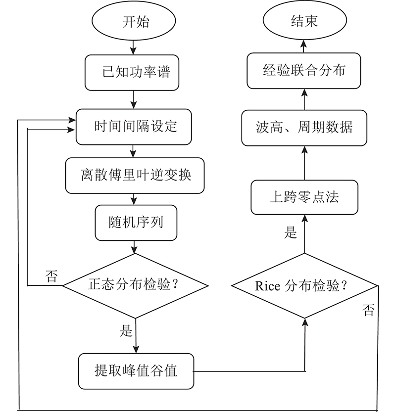
图 1 基于波浪谱的波高周期联合概率密度函数仿真流程图
Fig.1 Flow chart of joint probability density function of wave height and period based on wave spectrum
在得到满足要求的波面高程
3. 基于理论波浪谱仿真数据的对比分析
3.1. 理论波浪谱
式中:
可以推导出P-M谱的平均跨零周期表达式为
在已知有义波高的情况下,利用式(16)、(10)可以给出波高周期的联合概率密度函数.
根据式(15)可以推导出布氏谱的谱峰频率
在已知有义波高和平均跨零周期的情况下,根据式(18)、(10)可以给出波高周期的联合概率密度函数.
3.2. 模型有效性的判别方法
为了检验各模型与经验联合概率密度的匹配程度,基于均方根误差提出模型有效性判别方法,表达式为
式中:
3.3. 基于P-M谱仿真数据的对比分析
根据全球波浪数据GWS中的4个海区(8、9、15和16)长期统计资料进行仿真[14],有义波高取值范围为[0.5, 13.5] m. 根据式(19)计算各模型的RMSE,结果分别如图2和表1所示. RMSE数值随有义波高的增大而不断减小. 随着有义波高
图 2
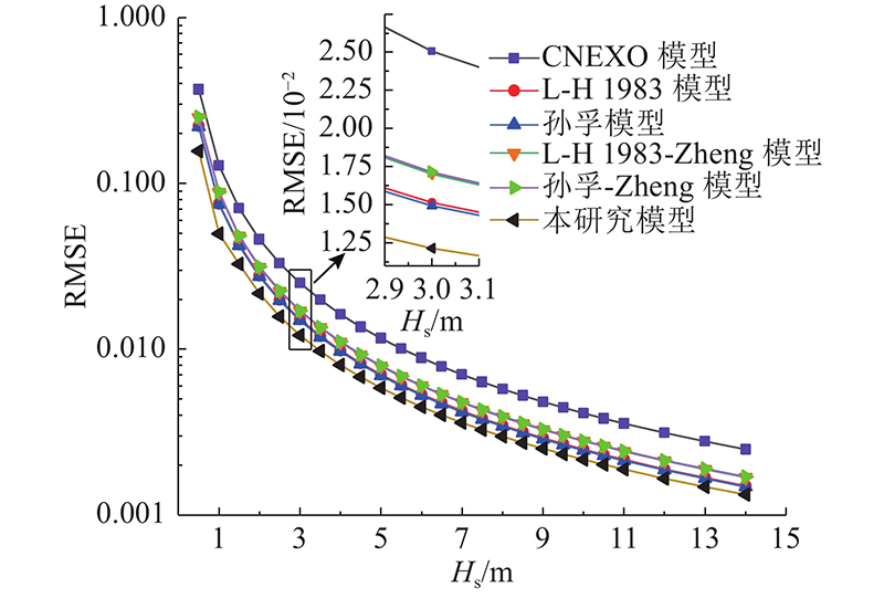
图 2 各模型均方根误差比较(P-M谱)
Fig.2 Comparison of root mean square error for each model (P-M spectrum)
表 1 各模型均方根误差数值(P-M谱)
Tab.1
| 模型 | RMSE | |||
| | | | | |
| CNEXO | 0.368 3 | 0.025 1 | 0.005 8 | 0.002 5 |
| L-H 1983 | 0.222 5 | 0.015 1 | 0.003 5 | 0.001 5 |
| 孙孚 | 0.219 6 | 0.014 9 | 0.003 4 | 0.001 5 |
| L-H 1983-Zheng | 0.249 9 | 0.017 0 | 0.003 9 | 0.001 7 |
| 孙孚-Zheng | 0.251 6 | 0.017 1 | 0.003 9 | 0.001 7 |
| 本研究 | 0.157 0 | 0.012 1 | 0.003 0 | 0.001 3 |
RMSE不能完全反映各模型在细节上的差异. 对比分析仿真结果与各模型概率密度函数发现,同一模型在不同海况中得到的结果相似. 选取
图 3
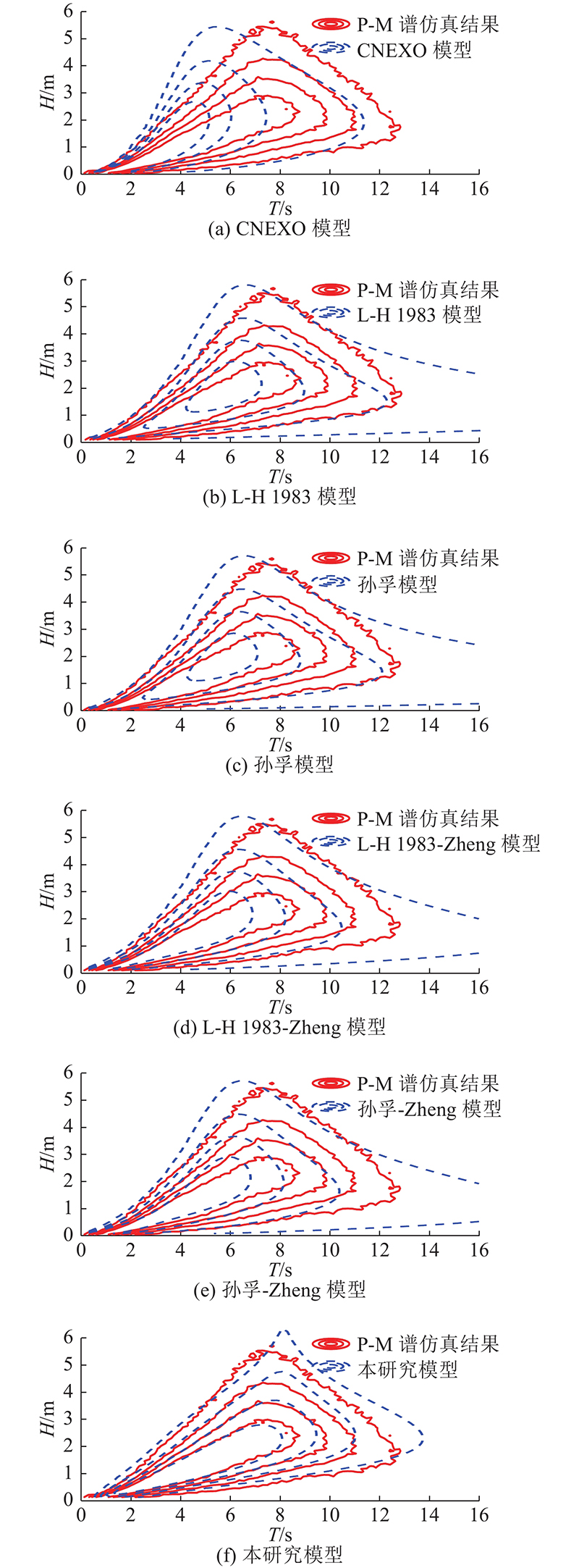
图 3 P-M谱仿真经验联合分布与各理论模型联合分布的比较(概率密度数值由外向内依次为0.001、0.010、0.030、0.060)
Fig.3 Comparison of empirical joint distribution of P-M spectrum simulation with joint distribution of each theoretical model (probability density values are 0.001, 0.010, 0.030, 0.060 in order from outside to inside)
图 4
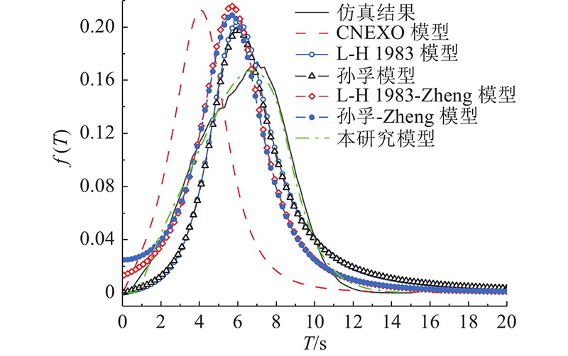
图 4 P-M谱仿真的周期概率分布与各模型的周期分布比较
Fig.4 Comparison of period probability distribution of P-M spectrum simulation with period distribution of each model
3.4. 基于布氏谱仿真数据的对比分析
表 3 各模型的均方根误差数值(布氏谱Hs=6 m)
Tab.3
| 模型 | RMSE | |||
| | | | | |
| CNEXO | 0.072 3 | 0.036 2 | 0.024 1 | 0.018 1 |
| L-H 1983 | 0.043 4 | 0.021 7 | 0.014 5 | 0.010 8 |
| 孙孚 | 0.042 8 | 0.021 4 | 0.014 3 | 0.010 7 |
| L-H 1983-Zheng | 0.048 6 | 0.024 3 | 0.016 2 | 0.012 2 |
| 孙孚-Zheng | 0.049 0 | 0.024 5 | 0.016 3 | 0.012 2 |
| 本研究 | 0.029 6 | 0.016 4 | 0.011 6 | 0.009 0 |
图 5

图 5 各模型的均方根误差比较 (布氏谱)
Fig.5 Comparison of root mean square error for each model (Bretschneider spectrum)
表 2 各模型的均方根误差数值(布氏谱Hs=0.5 m)
Tab.2
| 模型 | RMSE | |||
| | | | | |
| CNEXO | 2.630 5 | 0.375 8 | 0.175 4 | 0.105 2 |
| L-H 1983 | 1.588 7 | 0.227 0 | 0.105 9 | 0.063 6 |
| 孙孚 | 1.567 7 | 0.224 0 | 0.104 5 | 0.062 7 |
| L-H 1983-Zheng | 1.784 6 | 0.254 9 | 0.119 0 | 0.071 4 |
| 孙孚-Zheng | 1.796 8 | 0.256 7 | 0.119 8 | 0.071 9 |
| 本研究 | 0.834 5 | 0.162 4 | 0.084 5 | 0.054 3 |
表 4 各模型的均方根误差数值(布氏谱Hs=10 m)
Tab.4
| 模型 | RMSE | |||
| | | | | |
| CNEXO | 0.013 0 | 0.007 2 | 0.005 0 | 0.003 8 |
| L-H 1983 | 0.007 8 | 0.004 3 | 0.003 0 | 0.002 3 |
| 孙孚 | 0.007 7 | 0.004 3 | 0.003 0 | 0.002 3 |
| L-H 1983-Zheng | 0.008 7 | 0.004 9 | 0.003 4 | 0.002 6 |
| 孙孚-Zheng | 0.008 8 | 0.004 9 | 0.003 4 | 0.002 6 |
| 本研究 | 0.005 8 | 0.003 5 | 0.002 5 | 0.002 0 |
4. 基于实测波浪谱仿真数据的对比分析
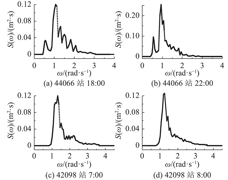
实测波浪谱与理论波浪谱存在差异. 为了进一步检验本研究模型的合理性,选取美国国家数据浮标中心2个不同浮标站具有代表性的4个实测波浪谱数据进行仿真分析. 实测波浪谱数据的基本情况如下. 1) 44066站(水深为78 m):2021年11月26日18:00数据,有义波高为1.1 m,谱峰周期为6 s,无涌浪情况;2021年11月26日22:00数据,有义波高为1.3 m,谱峰周期为7 s,无涌浪情况. 2) 42098站(水深为12 m):2021年11月27日7:00数据,有义波高为1 m,谱峰周期为5 s,无涌浪情况;2021年11月27日8:00数据,有义波高为1.1 m,谱峰周期为5 s,无涌浪情况. 将实测波浪谱数据绘图表示,如图6所示. 可以看出,实测波浪谱即使在仅风浪的情况下也会呈现出多峰形态,与经常使用的适用于风浪的单峰理论波浪谱有很大区别.
图 6
按照图6中的4个实测波浪谱进行仿真,并根据式(19)计算各模型的RMSE,结果如表5所示. 可以看出,对于每个实测波浪谱, CNEXO模型[8-9]的RMSE最大,本研究模型RMSE最小;L-H 1983模型和孙孚模型的RMSE接近,Zheng修正的2种模型的RMSE接近. 各模型的RMSE接近这一结论与2种理论谱仿真数据得出的结论一致. 由表5可以发现新的现象:对于42098浮标站的实测波浪谱,Zheng修正的2种模型[7]与仿真数据的匹配程度低于本研究模型、L-H 1983模型、孙孚模型. 对于44066浮标站的实测波浪谱,Zheng修正的2种模型与仿真数据的匹配程度仅次于本研究模型. 其中以44066浮标站实测波浪谱仿真数据所得出的结论与2种理论波浪谱得出的结论有差异.
表 5 各模型的均方根误差数值(实测谱)
Tab.5
| 模型 | RMSE44066 | RMSE42098 | |||
| 18:00 | 22:00 | 7:00 | 8:00 | ||
| CNEXO | 0.044 9 | 0.032 5 | 0.087 9 | 0.073 6 | |
| L-H 1983 | 0.040 5 | 0.030 9 | 0.070 2 | 0.059 1 | |
| 孙孚 | 0.040 4 | 0.030 6 | 0.070 0 | 0.058 8 | |
| L-H 1983-Zheng | 0.032 5 | 0.027 2 | 0.073 0 | 0.059 2 | |
| 孙孚-Zheng | 0.035 3 | 0.026 6 | 0.074 2 | 0.060 6 | |
| 本研究 | 0.031 1 | 0.026 8 | 0.049 1 | 0.047 8 | |
为了进一步确认RMSE对各联合模型与仿真数据匹配度的描述,同时确认周期T是影响各模型匹配度的主要因素,取44066站2021年11月26日18:00波浪谱仿真数据与各模型波高周期联合概率密度函数进行对比分析,结果如图7所示,与各模型周期T概率密度函数的比较如图8所示. 由图7、8可以发现,L-H 1983模型[5]、孙孚模型[6]存在大周期的情况,Zheng修正的2种模型[7]有效改善了这种情况,并在一定程度上提高了与仿真数据的匹配度. 结合图4、8可以发现,周期T概率密度函数的尾部(大周期)越接近仿真数据,模型的匹配度就越高. 由图7可以看出,L-H 1983模型[5]和孙孚模型[6]比较接近,Zheng修正的2种模型[7]比较接近. 这与2种理论波浪谱给出的结论一致. 分析结果表明,本研究模型无论是波高周期联合概率密度函数还是周期概率密度函数,都与仿真结果匹配较好.
图 7
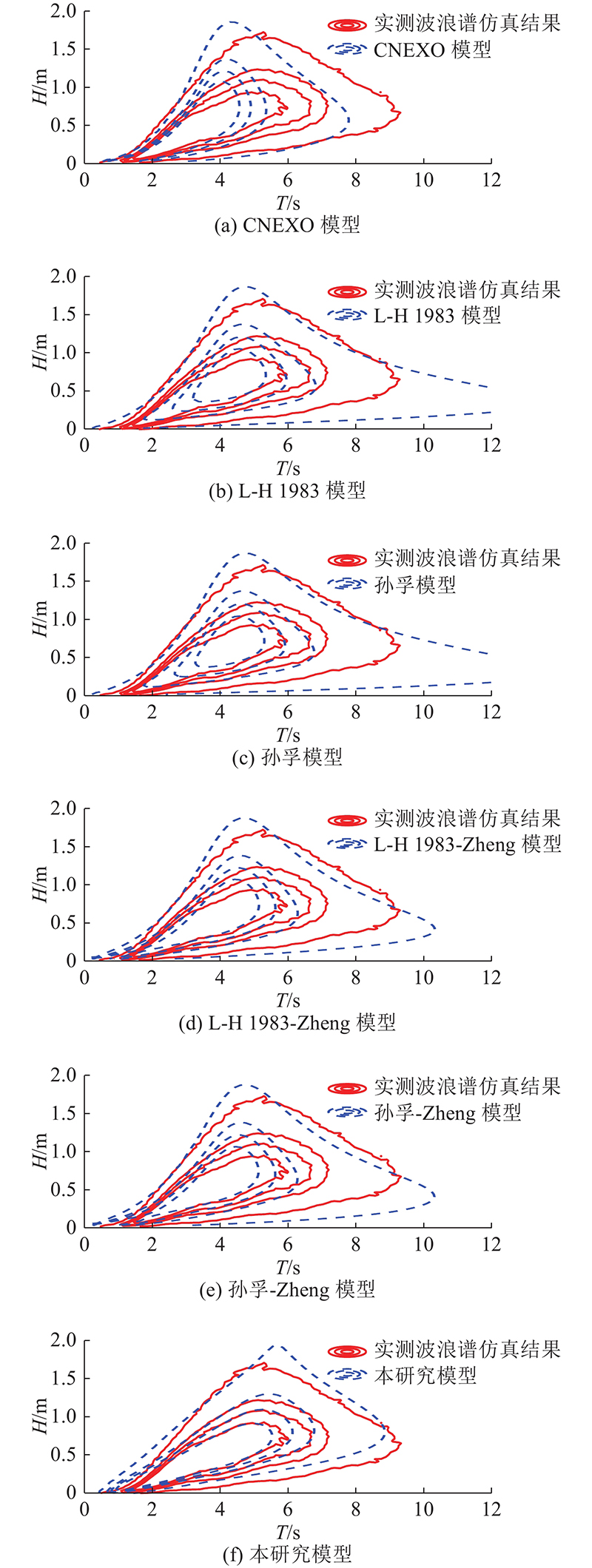
图 7 44066站实测波浪谱(18:00) 仿真经验联合分布与各模型联合分布的比较(概率密度数值由外向内依次为0.01、0.10、0.17、0.25)
Fig.7 Comparison of empirical joint distribution of measured wave spectrum simulation at 44066 station (18:00) with joint distribution of each model (probability density values are 0.01, 0.10, 0.17, 0.25 in order from outside to inside)
图 8
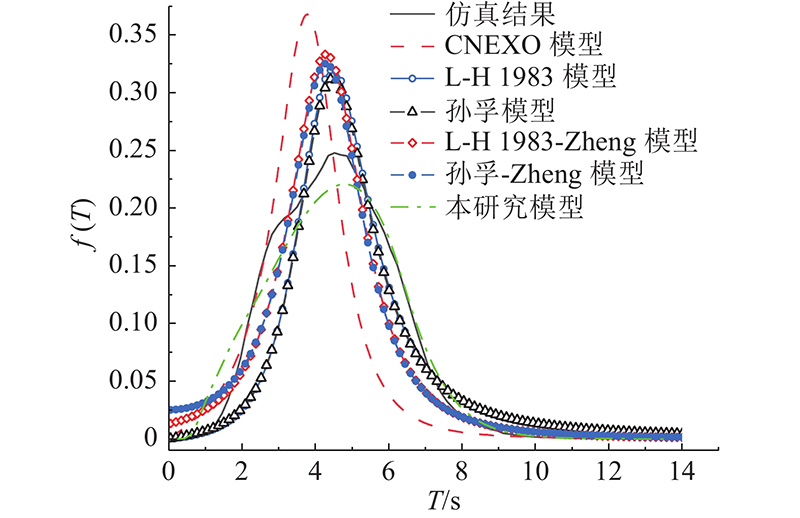
图 8 44066站实测波浪谱(18:00)仿真的周期概率密度分布与各模型的周期分布比较
Fig.8 Comparison of period probability distribution of measured wave spectrum simulation (18:00) at 44066 station with probability distribution of each model
5. 讨 论
在以上理论谱和实测谱的分析过程中发现,L-H 1983模型[5]和孙孚模型[6]分布形态比较接近. 这主要是由于这2种模型采用的方法基本相同,不同点仅在于对负角速度情况的处理上. 虽然2种模型的公式表达形式存在一定差异,但在数值上比较接近. 潘锦嫦等[10-11]对这2种模型进行分析后也得出类似结论. L-H 1983-Zheng模型、孙孚-Zheng模型因为提出者对模型进行了相同修正,所以在数值上比较接近. 对于深水情况,波浪谱的谱宽参数
6. 结 语
本研究提出新的短期风浪波高周期的联合分布模型,通过数值仿真验证了所提模型的准确性. 将所提模型与文献中常用的5种模型进行对比分析,得出以下结论:1) 本研究模型的精度较高,使用方便,但基于实测谱的计算精度略低于基于理论谱的计算精度;2) 由本研究模型推导出周期的概率密度函数具有较高的计算精度;3) L-H 1983模型的计算结果和孙孚模型的计算结果较接近,L-H 1983-Zheng模型的计算结果与孙孚-Zheng模型的计算结果较接近;4) L-H 1983-Zheng模型、孙孚-Zheng模型在短期风浪海况下,对波高周期联合分布的预报精度提高不明显. 此外,本研究模型可以推广到非高斯海况的应用场景中. 在后续的研究中,计划分析条件密度概率函数的一般表达公式,进一步提高模型的计算精度.
参考文献
On the joint distribution of the periods and amplitudes of sea waves
[J].DOI:10.1029/JC080i018p02688 [本文引用: 3]
On the joint distribution of wave periods and amplitudes in a random wave field
[J].
海浪周期与波高的联合分布
[J].
Joint distribution of wave period and wave height
[J].
The difference between the joint probability distributions of apparent wave heights and periods and individual wave heights and periods
[J].
海浪波高与周期联合概率密度分布的研究
[J].
Study of the joint probability density distribution of wave heights and periods
[J].
基于实测资料的南海海浪波高和周期联合分布研究
[J].
Study on the joint distribution of wave heights and periods in the south China sea based on observed data
[J].
Efficient FFT simulations of digital time sequences
[J].DOI:10.1061/JMCEA3.0002463 [本文引用: 1]
A modified straightforward spectral representation method for accurate and efficient simulation of the stationary non-Gaussian stochastic wave
[J].DOI:10.1016/j.oceaneng.2020.107308 [本文引用: 1]
Modelling and statistical analysis of ocean-wave data using transformed Gaussian processes
[J].DOI:10.1016/S0951-8339(96)00017-2 [本文引用: 1]
Analysis of ocean wave characteristic distributions modeled by two different transformed functions
[J].DOI:10.1007/s11804-019-00101-w [本文引用: 1]
